An abridged Javascript implementation is shown below.
To demonstrate the data structure in the web app, start with the following script.
let f = new Forest();
f.fromString('{a(b(c d) e(f(g)) h) i(j k(l m) n)}');
f.cut(5); f.combineGroves(1,9);
log(f.toString());
The $\fromString$ operation specifies two trees with roots $a$ and $i$.
In the string argument, each node is shown with its descendants
immediately following it, enclosed by paretheses.
So, initially $a$ has children $b$, $e$ and $h$, with the first two
each defining subtrees with two additional descendants.
The $\cut$ operation removes $e$'s subtree from $a$ and the
$\combineGroves$ operation pairs $i$'s tree with the remainder of $a$'s tree
to form the grove shown below.
{[a(b(c d) h) i(j k(l m) n)] e(f(g))}
Adding
f.cut(11) f.link(11,6);produces
{[a(b(c d) h) i(j n)] e(f(g k(l m)))}
Adding an argument of 0 to the $\toString$ method causes it to
omit the tree structure, showing each grove or stand-alone tree
as just a list of vertices in prefix order.
{[a b c d h i j n] [e f g k l m]}
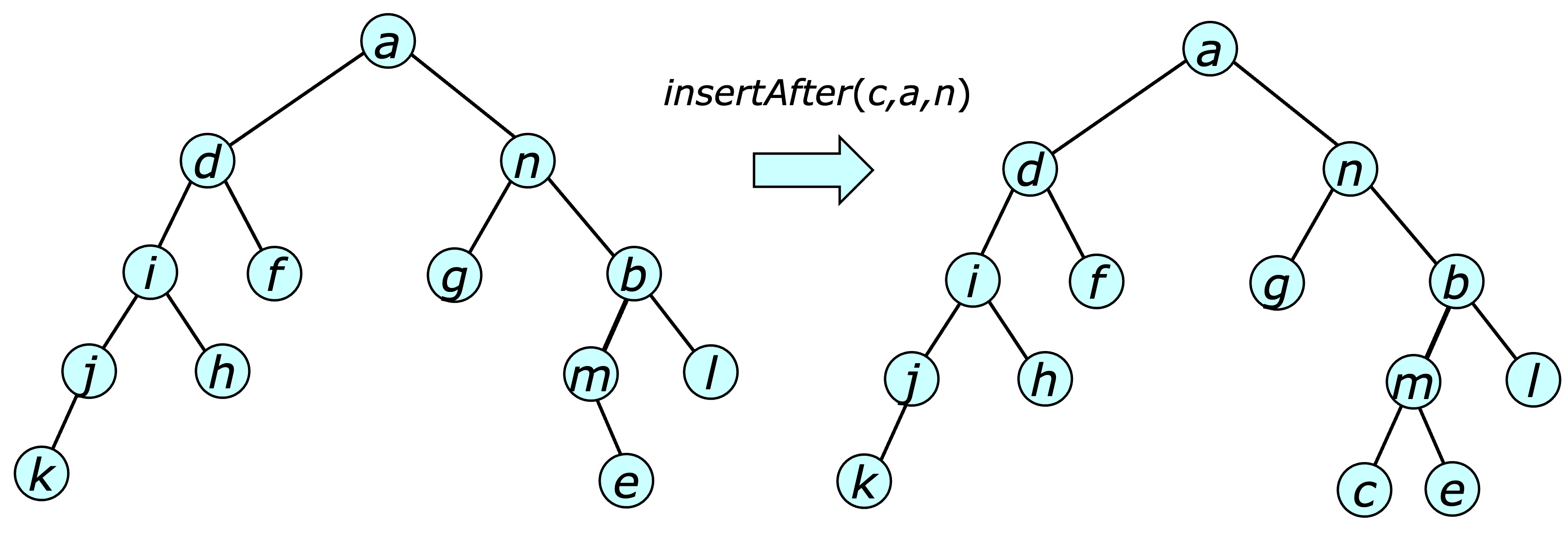
The inserted vertex $c$ becomes the leftmost leaf in the right subtree of its specified predecessor $n$.
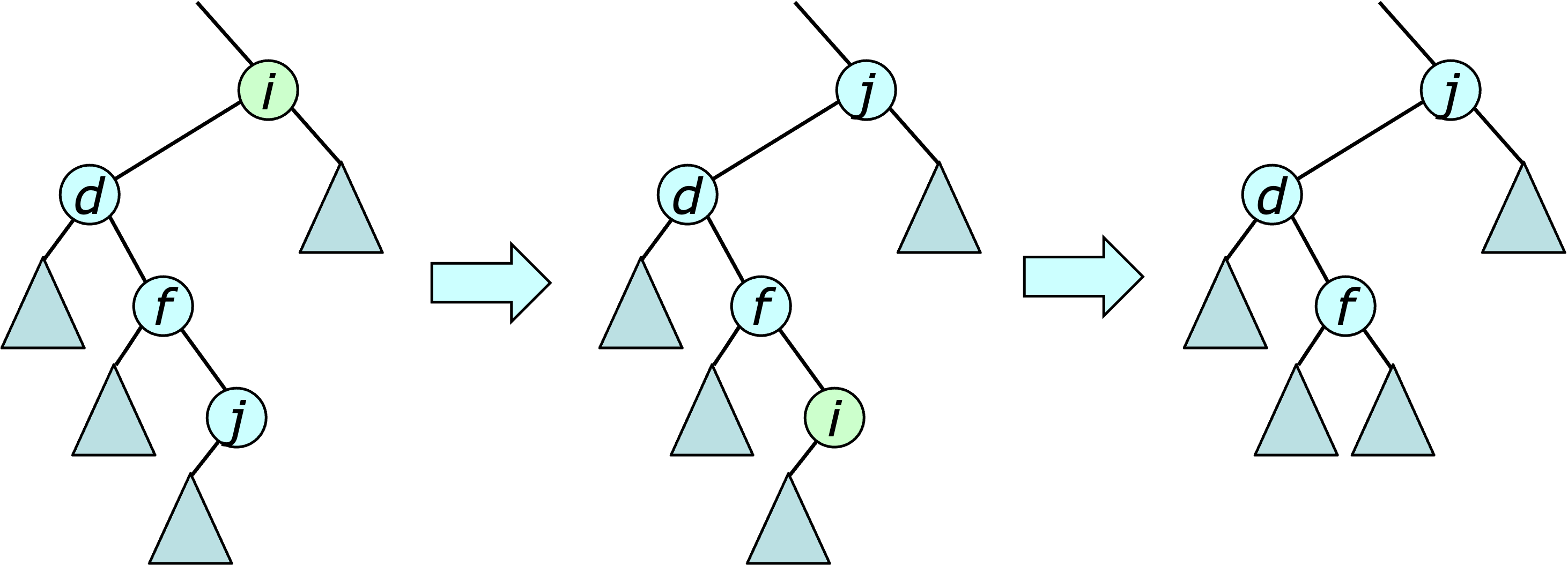
Deleting a vertex $v$ from a tree is easy if $v$ has no children. Just cut the link to its parent. It is almost as easy if $v$ has one child, since that child can simply take $v$'s place in the tree. If $v$ has two children, its position in the tree is first swapped with the “rightmost vertex” in its left subtree. This vertex is its immediate predecessor in the tree. At that point, it has at most one child, making the deletion easy. This is illustrated below.
The operation $\join(t_1,u,t_2)$ operation is easy. Simply make $t_1$ the left child and $t_2$ the right child of $u$. The operation $\split(u)$ operation is similarly easy if $u$ is a tree root. If not, the split is accomplished by starting at item $u$ and proceeding up the tree, building two subtrees $L$ and $R$ where $L$ contains the vertices to the left of $u$ and $R$ contains the vertices to its right. This is illustrated below.
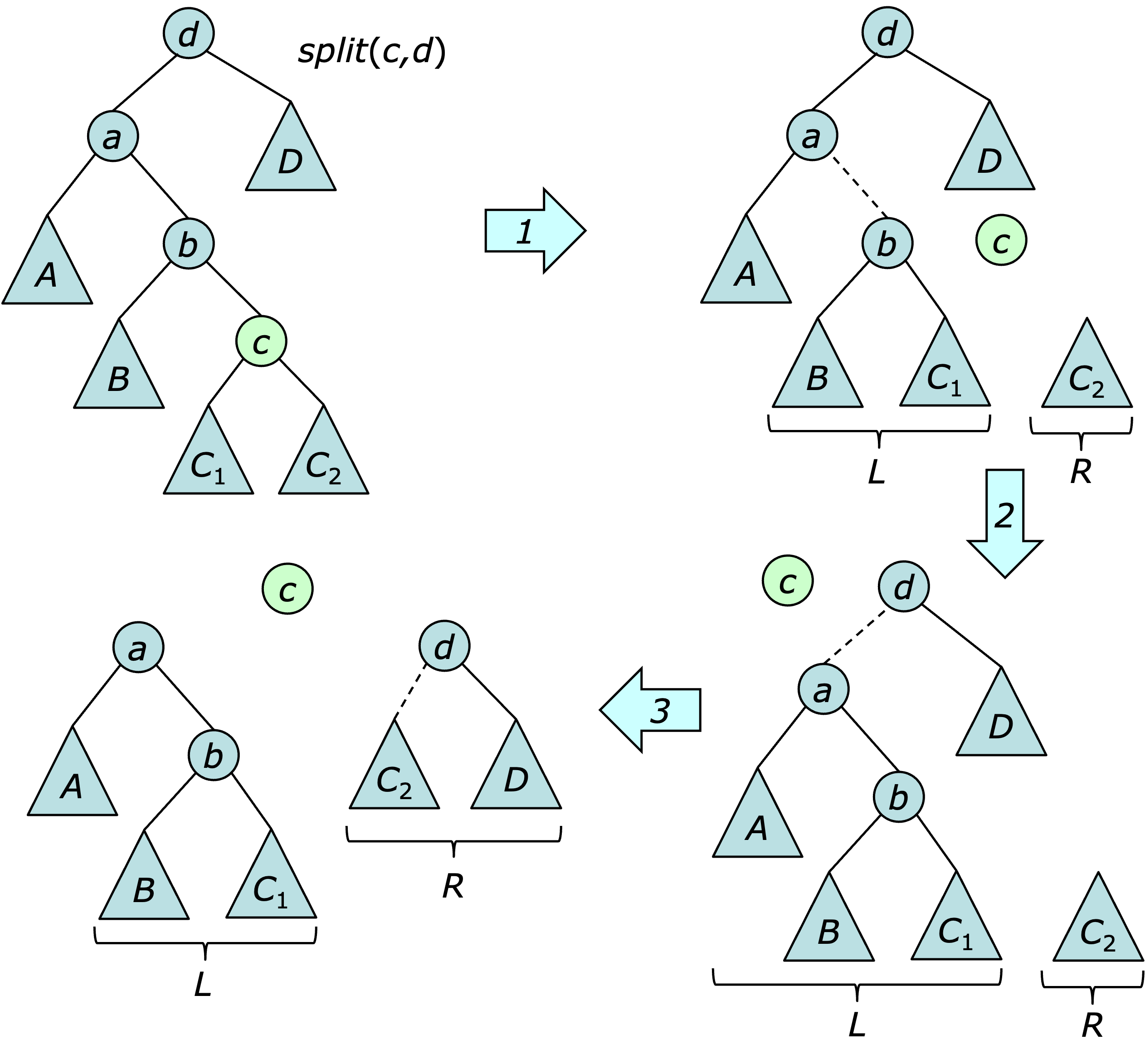
Observe that the first step completes a split of the subtree of vertex $c$'s parent $b$. The next step completes a split of the next subtree up the path to the root. The third completes the split for the whole tree.
Binary trees are often used to implement search trees in which each vertex $u$ is assigned a value $\key[u]$ and the left-to-right order of the search tree vertices matches the increasing order of the key values, as illustrated below.
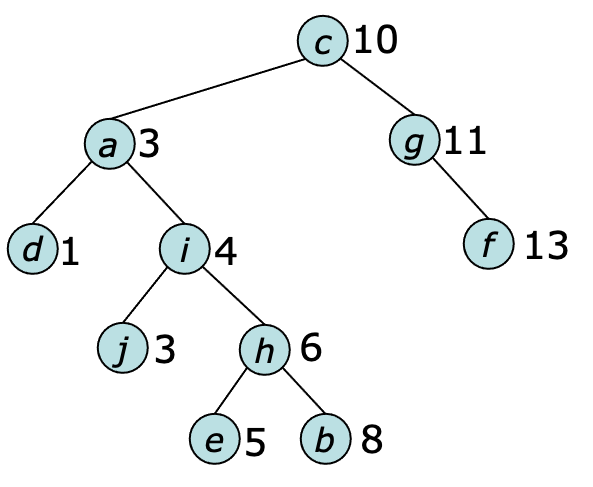
The operation $\search(k,t,key)$ uses the provided key values to locate a vertex with the specified key. It starts at the root and at each step compares the key of the current vertex with that of $u$. In the example above $\search(5,c,key)$ follows the path $[c,a,i,h,e]$ from the root, at each step comparing the key of the current vertex to the target key value and selecting the left or right subtree based on that comparison.
The operation $\insertByKey(u,t,key)$ is intended for use in this situation. It starts by using the provided keys to find a location where $u$ can be inserted as a new leaf, while ensuring that the order of the tree's vertices remains consistent with the key values. In the example above, if $\key[m]=7$ the operation $\insertByKey(m,c,key)$ would search the tree looking for a viable location, eventually inserting $m$ as the right child of $e$.
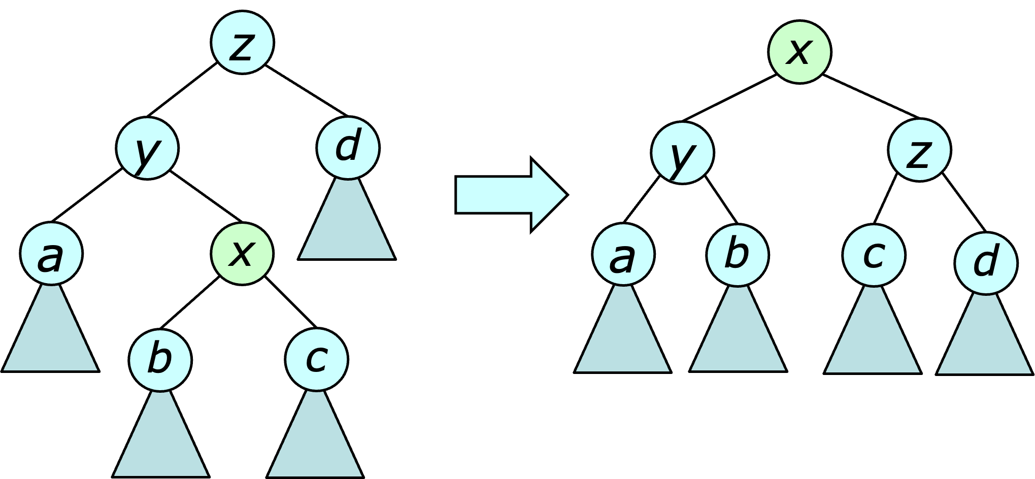
The operation $\rotate(x)$ is illustrated below.

Notice that the operation moves $x$ one step closer to the root and moves its parent one step further away. If applied in a systematic fashion, rotations can be used to reduce the maximum depth of a tree. In particular, the $\BalancedForest$ data structure (see next sub-section) uses rotations to ensure that the tree depth is never more than twice the log of the tree size.
Rotations are often used in pairs. In particular, when $x$ is an outer grandchild, a double-rotation at $x$ consists of a first rotation at its parent, then a rotation at $x$, as illustrated below.

When $x$ is an inner grandchild, both rotations are done at $x$.
An abridged Javascript implementation appears below.
Notice that most methods that modify a tree's structure provide an optional function argument called $\refresh$. These functions can be used to assist in balancing the data structure, and/or maintaining client data that may be affected by the tree structure.
To demonstrate the data structure, start with the following script.
let bf = new BinaryForest();
bf.fromString('{[(a b -) *c (d e f)] [(g h (- i j)) *k l] [m *n (o p r)]}');
bf.insertAfter(17,11,8);
log(f.toString()); log(f.toString(0));
The $\fromString$ operation specifies three trees with roots $c$, $k$ and $n$.
Note that in this case, each tree is surrounded by square brackets and the
roots are highlighed with an asterisk
(brackets are omtted for single vertex trees).
Also, for any non-leaf node a
“missing child” is shown explicitly.
The $\insertAfter$ operation inserts $q$ in the tree with root $k$,
just after $h$.
The $\toString$ operations produce the output below.
{[(a b -) *c (d e f)] [(g h (q i j)) *k l] [m *n (o p r)]}
{[a b c d e f] [g h q i j k l] [m n o p r]}
Adding
bf.split(9); bf.join(3,9,14);divides the tree containing $i$ into three parts and then joins the trees with roots $c$ and $n$ to $i$. This yields
{[((a b -) c (d e f)) *i (m n (o p r))] [g *h q] [j *k l]}
Adding two rotate operations at $e$ produces
{[((a b -) c d) *e (f i (m n (o p r)))] [g *h q] [j *k l]}
The $\BalancedForest$ data structure is designed to handle such applications efficiently by limiting the depth of its trees to at most $2\lg n $. There are many ways to keep trees balanced. The $\BalancedForest$ uses a method described in [Bayer72, Tarjan87], which assigns a $\rank$ to every node, and ensures that the ranks satisfy two properties. $$ \rank(u) \leq \rank(p(u)) \leq \rank(u) +1 \\ \rank(u) < \rank(p^2(u)) $$ where $p^2(u)$ is the grandparent of $u$. Vertices with fewer than two children are assigned a rank of 1. An example of such a tree is shown below.
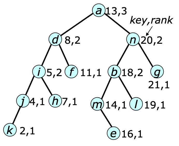
One can show by induction that any node of rank $k$ has height at most $2k-1$ and has at least $2^k-1$ descendants. This implies that the maximum depth of any node is $\leq 2 \lfloor\lg (n+1)\rfloor$.
Operations that modify a tree must be extended to to ensure that the conditions on the ranks are maintained. Following an insertion of a node $x$, one must compare $\rank(x)$ with $\rank(p^2(x))$. If $\rank(x)$ is smaller, nothing further needs to be done. If the two ranks are equal, but $x$'s aunt (the sibling of its parent) has smaller rank, the rank conditions can be satisfied by doing one or two rotations. Specifically, if $x$ is an outer grandchild, a single rotation at $p(x)$ completes the process. If $x$ is an inner grandchild, a double-rotation at $x$ is required. This is illustrated below.

If $\rank(x)=\rank(p^2(x))=\rank(\aunt(x))$, $\rank(p^2(x))$ is incremented and the checking procedure is repeated at $p^2(x)$
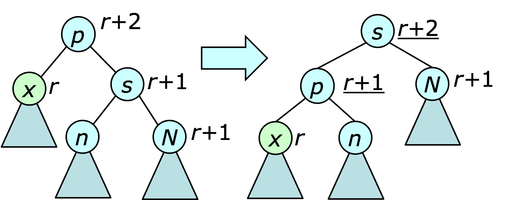
The procedure for balancing after a deletion is a bit more involved. It starts at the vertex $x$ that took the place of the deleted node. Let $r$ be its rank. There are four case to consider. (Case 1) If $x$'s parent has rank $r+2$ then there is a violation of the first rank condition that needs to be fixed. If $x$'s sibling also has rank $r+2$, a rotation is performed at the sibling, as illustrated below.
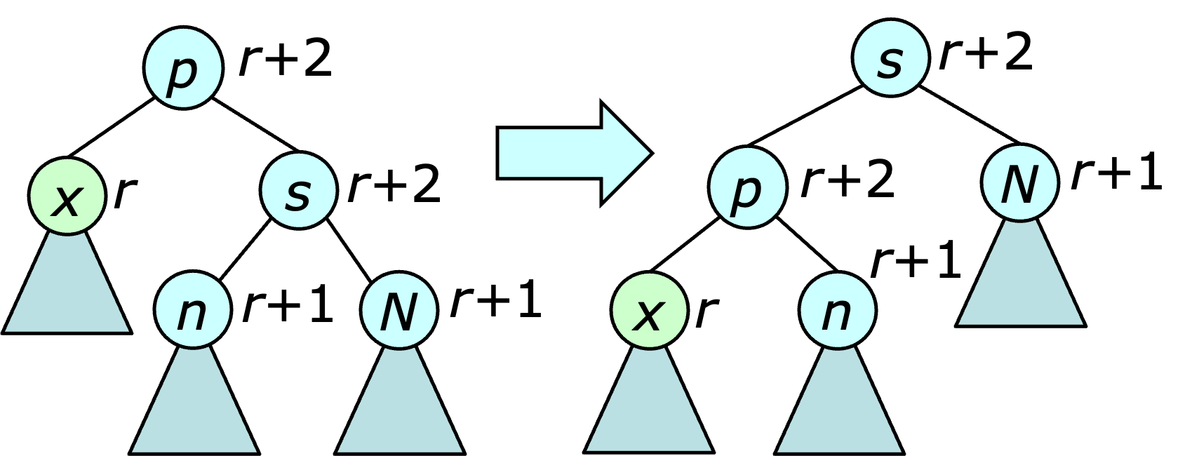
This rotation does not fix the rank violation at $x$, but because $x$'s new sibling has rank $r+1$, the violation can now be addressed using one of the three remaining cases.
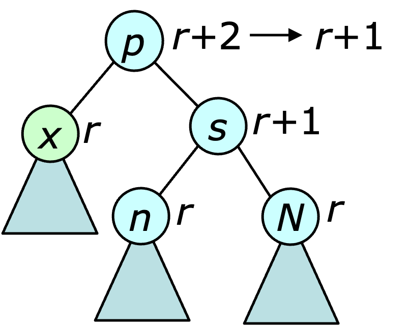
(Case 2) If $x$'s sibling has rank $r+1$ and both of its children have rank $r$, then $\rank(p(x))$ is decremented, eliminating the rank violation at $x$, but possibly creating a new violation between $p(x)$ and its parent. In this case, the checking procedure is repeated, with $p(x)$ replacing $x$.
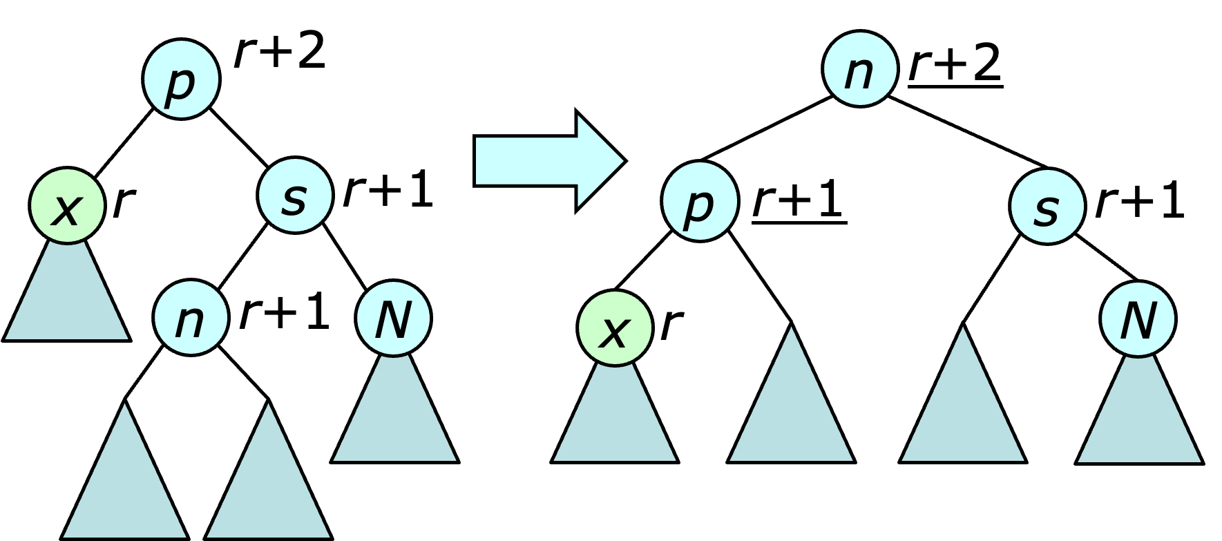
(Case 3) If $x$'s sibling has rank $r+1$ and $x$'s nephew (the more distant child of $x$'s sibling) has rank $r+1$, a rotation is performed at the sibling and the ranks of $x$'s parent and its new grandparent are changed to $r+1$ and $r+2$ respectively.
(Case 4) Finally, if $x$'s sibling has rank $r+1$ and its niece has rank $r+1$, a double rotation is performed at the niece and the ranks of $x$'s parent and grandparent are changed to $r+1$ and $r+2$.
Note that the last two cases eliminate the violation at $x$ and create no new violations, so the rebalancing process ends at that point. Also, if an application of the first case is followed by an application of the second case, there can be no remaining violation of the rank condition at that point.
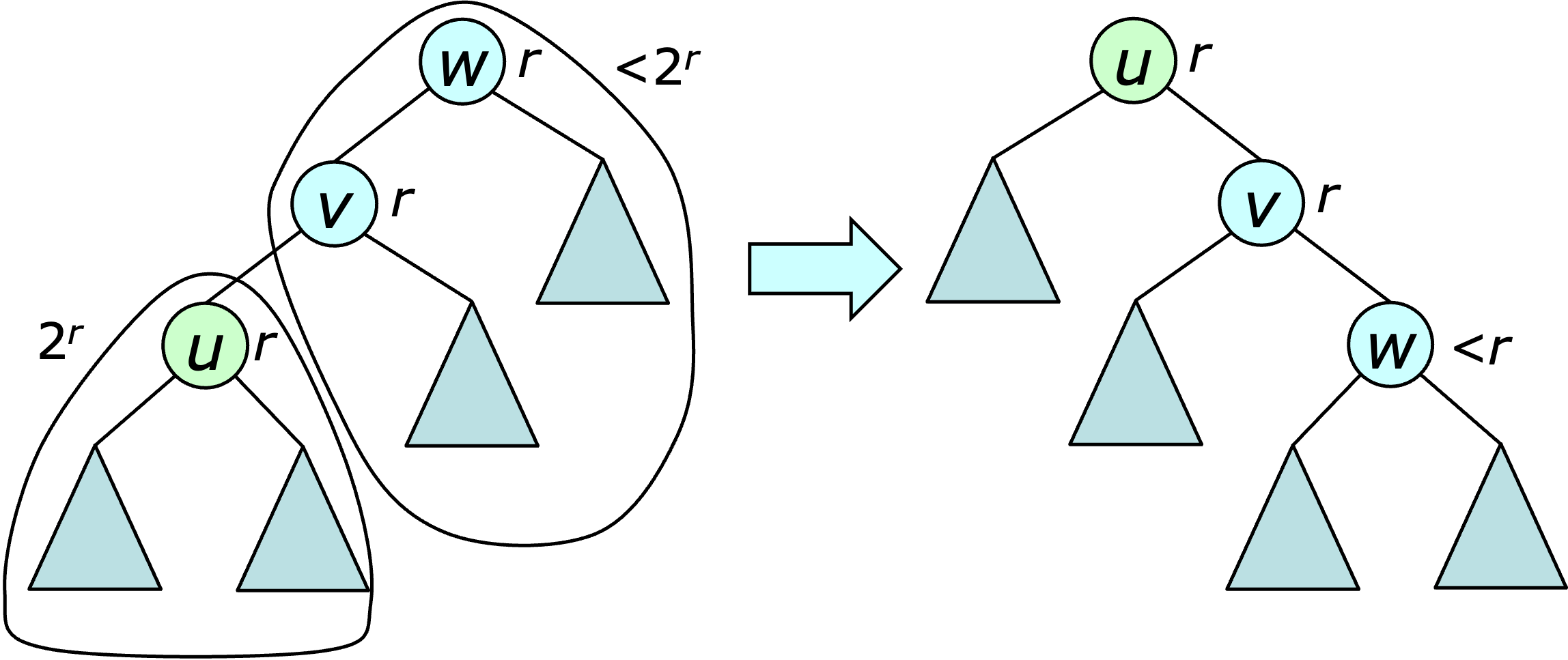
The operation $join(t_1,i,t_2)$ can be performed as before, if $\rank(t_1)=\rank(t_2)$. In this case, $\rank(i)$ is set to $\rank(t_1)+1$. If $\rank(t_1) \neq \rank(t_2)$, things get more complicated. If $\rank(t_1) > \rank(t_2)$, the first step is to follow right pointers from $t_1$ looking for the first vertex $v$ with $\rank(v)=\rank(t_2)$. The subtree at $v$ is then joined to $i$ and $t_2$ and the resulting subtree takes the original place of $v$ in $t_1$. This is illustrated below.
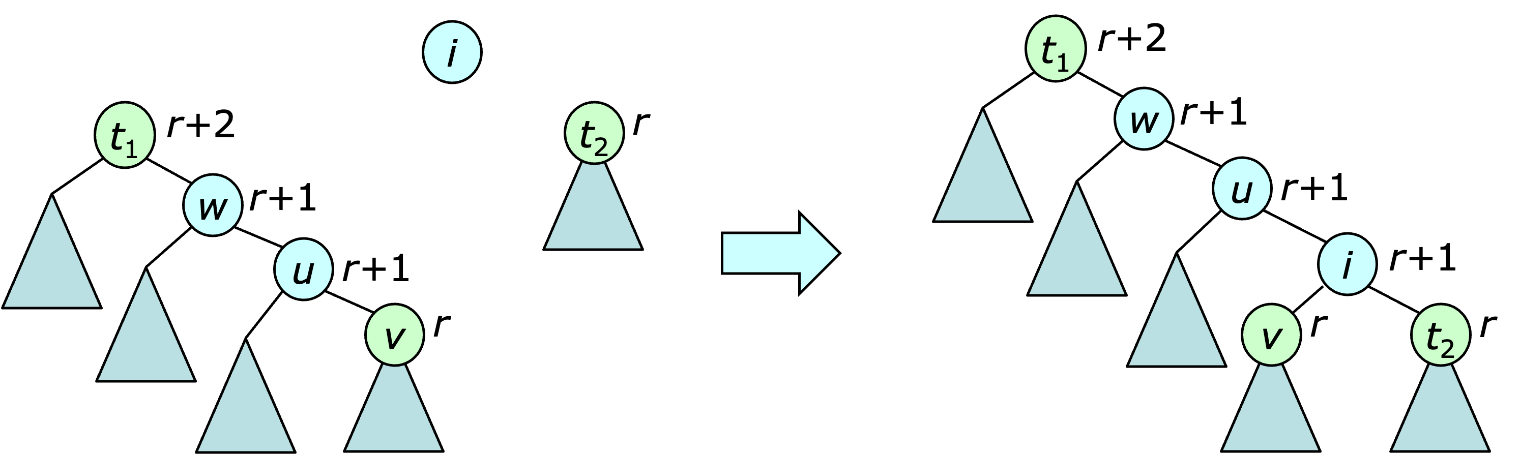
Since this procedure may produce a violation of the second rank condition, the rebalancing procedure used for inserts is applied at this point, starting at $i$.
The split operation is done as before, but uses the balanced version of the join operation in place of the original.
Here is the abridged Javascript implementation.
Observe how the $\refresh$ function arguments are used to implement the re-balancing.
To demonstrate the data structure, start with the following script.
let bf = new BalancedForest();
bf.fromString('{[a b c d e] [h i j k l m n o p q r]}');
log(bf.toString(0xc));
The $\fromString$ operation specifies two lists that are implemented as
trees by the data structure. Vertices that do not appear in either list
($f$ and $g$, in the example) are treated as singleton lists.
However, with the inclusion of the appropriate format argument,
the $\toString$ method can show the detailed tree structure as shown below.
{[(a b c) *d:2 e] [(h i:2 j) *k:3 (l m:2 ((n o p) q:2 r))]}
Note that ranks of one are omitted.
Adding the operations
let [t1,t2] = bf.split(15); bf.join(4,15,t1);splits the second tree at $o$ and then joins the tree with root $d$ to the first tree produced by the $\split$ yields
{[(((a b c) d:2 e) o:3 (h i:2 j)) *k:3 (l m:2 n)] [p *q:2 r]}
Deleting $d$ from the first tree yields
{[(((a b -) c:2 e) o:3 (h i:2 j)) *k:3 (l m:2 n)] [p *q:2 r]}
and re-inserting it after $a$ in the second tree yields
{[(((a d b) c:2 e) o:3 (h i:2 j)) *k:3 (l m:2 n)] [p *q:2 r]}
The key to this approach is a restructuring operation called a splay. A splay at a vertex $u$ consists of a series of double rotations at $u$, that moves $u$ to the root, or at most one step away. If needed, a final single rotation is used to bring $u$ to the root. An example is shown below.
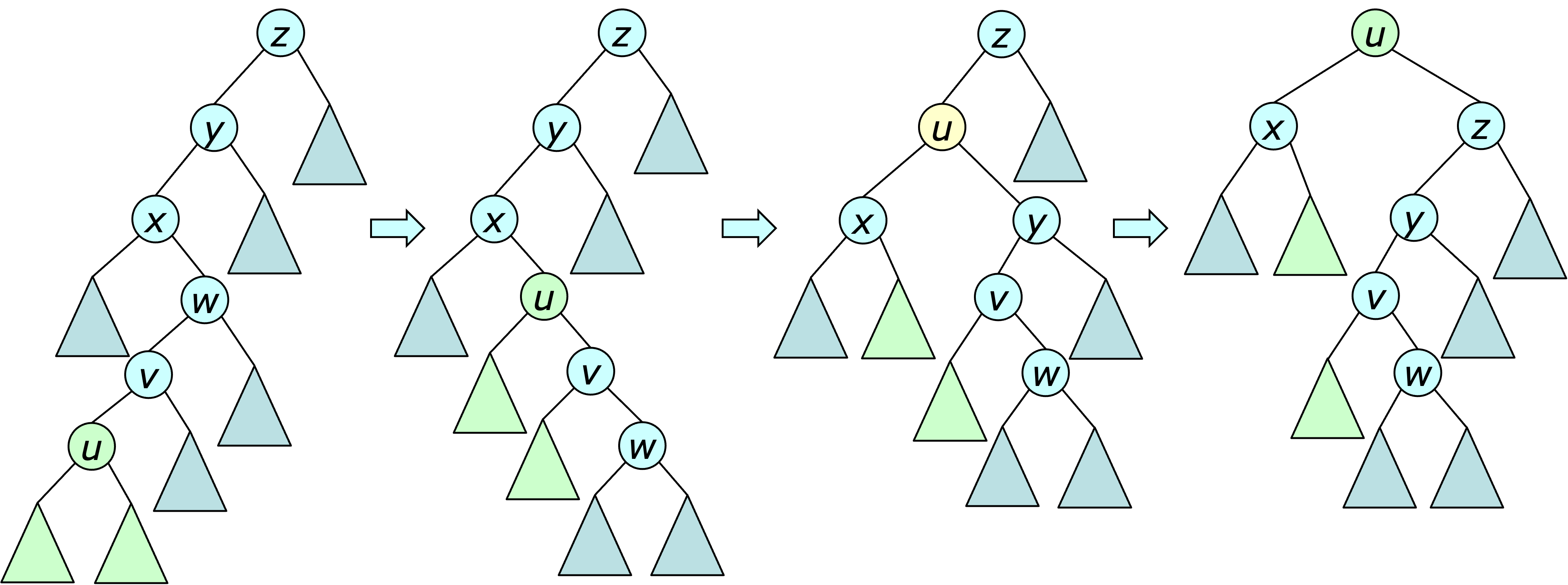
To understand why the splay is helpful, observe that any double-rotation at a node $u$ brings all descendants of $u$ at least one step closer to the root of the search tree. Consequently, if the nearest common ancestor of $u$ with a node $v$ has depth $d$ before the splay, then after the splay, the depth of $v$ is reduced by at least $\lfloor d/2 \rfloor -2$. For ancestors of $u$, this implies that their depth is roughly halved by the splay operation. Also note that the more expensive the splay is, the greater benefit it delivers.
When a search operation reaches a vertex with the target key value, a splay is performed at that vertex, improving the performance of future operations while only increasing the cost of the search by a constant factor. Similarly, a splay is performed after a vertex is inserted or deleted. No splay is performed during a join, but a split is implemented by first performing a splay at the split vertex $u$ and then simply separating the two subtrees of the new root, $u$.
An amortized complexity analysis can be used to show that the time required to do a sequence of $m$ operations on a collection of splay trees is $O(n + m\log n)$ or $O(m\log n)$ in the common case where $m\geq n$. The analysis uses a set of fictitious “credits” that are allocated for each operation and used to “pay” for computational steps. Credits that are not needed to pay for a particular operation can be saved and used to pay for later operations. The total number of credits allocated to a sequence of operations then serves as an upper bound on the number computational steps. To ensure that there are always enough credits on hand, credits are allocated so as to satisfy the following credit policy.
For each vertex of $u$, maintain $\rank(u)= \lfloor \lg (\textrm{the number of descendants of }u)\rfloor$ credits.
To determine the number of credits that must be allocated to a splay operation at vertex $u$, let's first determine the number needed for one double-rotation. Let $v$ be the parent of $u$ and $w$ its grandparent and let $\rank'$ denote the rank values after the rotation (note that $\rank'(u)=\rank(w)$). The number of credits needed to satisfy the credit policy following a double rotation is \begin{eqnarray*} (\rank'(u)-\rank(u)) &+& (\rank'(v)-\rank(v)) + (\rank'(w)-\rank(w)) \\ &=&(\rank'(w)+\rank'(v)) - (\rank(u)+\rank(v)) \\ &\leq& 2(\rank(w) - \rank(u)) \end{eqnarray*} If $\rank(u) < \rank(w)$ and $3(\rank(w) - \rank(u))$ credits are allocated for the double rotation, there will be at least one credit available to pay for the operation, while still satisfying the credit policy.
Now consider the case where $\rank(u)=\rank(w)=r$. If $u$ is an inner grandchild, then after the double-rotation, $v$ and $w$ are its children, meaning that at least one of them has a smaller rank after the operation. This implies that there is one less credit needed to satisfy the credit policy after the operation, and this credit can be used to pay for it. If $u$ is an outer grandchild, then $u$ has at least $2^r$ descendants and $w$ has fewer than $2^r$ descendants outside of $u$'s subtree. This implies that after the operation $w$ has fewer than $2^r$ descendants, making $\rank'(w) < r$.
So again, one less credit is needed to satisfy the credit policy and that credit can be used to pay for the operation. Summarizing, if $3(\rank(w)-\rank(u))$ credits are allocated to each double rotation, the operation can be paid for while continuing to satisfy the credit policy.
If a single rotation is required to complete a splay, the number of credits needed to satisfy the credit policy after the operation is $$ (\rank'(u)-\rank(u)) + (\rank'(v)-\rank(v)) =\rank'(v) - \rank(u) \leq \rank(v) - \rank(u) $$ If $3(\rank(v) - \rank(u))+1$ credits are allocated for the rotation, it can be paid for while still satisfying the credit policy. These observations are summarized in the following lemma.
Lemma. Let $u$ be a vertex in a tree with root $v$. If $3(\rank(v)-\rank(u))+1$ credits are allocated to a splay operation at $u$, the operation can be fully paid for while continuing to satisfy the credit policy.
Note that this implies that at most $3\lfloor \lg n \rfloor+1$ credits are needed for each splay. The next step in the analysis of splay trees is to determine the number of credits that must be allocated to each operation in addition to those required for splays. For an insert operation, each vertex along the path from the inserted vertex to the root acquires a new descendant and consequently, the ranks will increase for those vertices that have exactly $2^k-1$ descendants before the insertion. There are at most $\lfloor \lg n \rfloor+1$ such vertices, so the total number of credits needed for the insert (including the splay) is $\leq 4(\lfloor \lg n \rfloor)+3$.
The join requires an additional $\lfloor \lg n \rfloor+1$ credits to satisfy the credit policy at the new tree root, and since no splay is involved, $\lfloor \lg n \rfloor+2$ credits are sufficient to pay for the operation while continuing to satisfy the credit policy.
The other operations require just one credit beyond those needed for the splay, so the total number of credits required for $m$ operations is $O(m\log n)$. The initialization can be paid for with $n$ credits and no additional credits are needed to satisfy the credit policy initially. Since every operation is paid for with allocated credits and the number of credits allocated is $O(n + m \log n)$, the time required for the operations is also $O(n + m \log n)$.
The splay lemma is also true using a more general definition of the $\rank$. Specifically, if each vertex $u$ is assigned some arbitrary weight $w(u)$ and $tw(u)$ is defined as the total weight of the subtree with root $u$, then $\rank(u)$ can be defined as $\lfloor \lg tw(u) \rfloor$. The argument used earlier still works with this definition. The more general version is used in a later chapter to analyze the performance of the dynamic trees data structure.
An abridged Javascript implementation is shown below.
To demonstrate splay trees, run the following script.
let sf = new SplayForest();
sf.fromString('{[((((((((a b -) c -) d -) e -) f -) g -) h -) i -) *j -]}');
sf.splay(1); log(sf.toString());
sf.splay(3); log(sf.toString());
sf.splay(5); log(sf.toString());
The $\fromString$ operation creates a highly unbalanced tree
and each splay improves the balance, as shown below.
{[- *a (((((- b c) d e) f g) h i) j -)]}
{[(- a b) *c (((- d e) f (g h i)) j -)]}
{[((- a b) c d) *e ((- f (g h i)) j -)]}
In most situtions, balanced binary trees are more efficient than
splay trees, since they requires far fewer rotations.
While a single rotation does take constant time, it is a
fairly expensive operation.
Still, there are some situations where splay trees can out-perform
explicitly balanced trees.