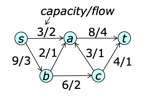
An example of a graph with a flow is shown below.
The sum of the flows leaving $s$ is referred to as the value of the flow and is denoted $|f|$. The objective of the maximum flow problem is to find a flow function with the largest possible value. In principle, edge capacities may be real numbers, but in practice, the use of floating point values to represent capacities can lead to numerical issues. Restricting capacities and flows to integer values eliminates this concern.
Define a cut to be a partition of $V$ into two parts $X$ and $Y$ with $s\in X$ and $t\in Y$. The capacity of the cut is $cap(X,Y)$. The flow across the cut is $f(X,Y)$. A cut of minimum capacity is called a minimum cut. The dashed line in the diagram below defines a minimum cut.

The flow conservation property implies that for any cut $(X,Y)$, $f(X,Y)=|f|$. To prove this, note that $$ f(X,Y) = f(X,V) - f(X,X) $$ By skew symmetry, the second term is zero, so $$ f(X,Y) = f(X,V) = f(s,V) + f(X-s,V) = |f| + \sum_{u \in X-s} f(u,V) = |f| $$ where the last equality follows by flow conservation. The capacity constraint implies that for any flow $f$ and any cut $(X,Y)$, $f(X,Y) \leq cap(X,Y)$. This implies that the maximum flow value is no larger than the capacity of a minimum cut. The max-flow, min-cut theorem states that the maximum flow value is equal to the minimum cut capacity.
Before verifying this, let's first define the residual capacity of an edge $e=(u,v)$ as $\res_e(u,v) = cap_e(u,v) - f_e(u,v)$ and $\res_e(v,u)=f_e(u,v)$ ($=cap_e(v,u)-f_e(v,u)$). The residual capacity gives the amount by which flow can be increased in either the forward or reverse direction on an edge, without violating capacity constraints. For non-adjacent vertices $u$ and $v$, $\res(u,v)=0$.
For any vertex pair $u$ and $v$, define a flow path to be any path from $u$ to $v$ consisting of edges in either orientation. The residual capacity of a flow path from $u$ to $v$ is the minimum residual capacity of its edges, in the $u$-to-$v$ direction. So in the previous example, the edges $(b,a)$ and $(b,c)$ define a flow path from $a$ to $c$ with residual capacity 1, with the first edge being traversed in the reverse direction. An edge or flow path with a residual capacity of 0 is said to be saturated. If there is a flow path from $u$ to $v$ with positive residual capacity, then $v$ is said to be reachable from $u$. Note that if $t$ is reachable from $s$, then flow can be added to some $s$-$t$ path. Such a path is called an augmenting path.
Now, suppose $f$ is a maximum flow. Let $X$ be the set of vertices reachable from $s$ and note that $t\not\in X$, since if it were, more flow could be added from $s$ to $t$. Consequently $(X,Y)$ defines a cut and every edge crossing the cut must be saturated in the direction from $X$ to $Y$. Consequently, $|f|=f(X,Y)=cap(X,Y)$. Since $|f|$ is bounded by the capacity of every cut, there can be no cut with a smaller capacity, hence $(X,Y)$ is a minimum cut, confirming the max-flow, min-cut theorem.
Select an augmenting path $p$ and add $\res(p)$ units of flow to all edges on $p$.
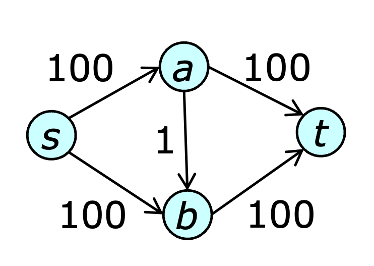
This method was first proposed by Ford and Fulkerson [FF56]. If flow capacities are integers, flow increases by at least 1 on each step, so the augmenting path algorithm terminates in at most $|f^\ast|$ steps, where $f^\ast$ is a maximum flow. The figure below shows a graph in which the augmenting path method could alternate between the paths $[s,a,b,t]$ and $[s,b,a,t]$ taking 200 steps to arrive at a maximum flow.
Efficient algorithms can be obtained using an appropriate path selection policy. There are two natural choices, both suggested by Edmonds and Karp [EK72]. The first is to select augmenting paths of minimum length (where path length is simply the number of edges in the path). The second is to select paths of maximum residual capacity. Both of these algorithms use just two steps to find a max flow in the example graph.
As usual, the code has been abridged for clarity. The complete version includes execution tracing and performance statistics. Notice that the inner for loop of the findpath function iterates over all edges incident to vertex $u$, both incoming and outgoing.
The following script can be used to run the program in the web app.
let g = new Flograph();
g.fromString('{a->[b:3 d:2] b[c:3 d:7 g:3] c[d:1 e:5] d[e:2 f:1 g:3] ' +
             'e[f:1 g:3 h:4] f[e:1 g:2 h:3] g[e:3 f:2 h:1] ' +
             'h[f:3 i:4 j:2] i[g:5 j:6] ->j[]}');
let [ts] = maxflowFFsp(g,1);
log(ts);
This produces the output
augmenting paths with residual capacities
a:3 b:3 g:1 h:2 j
a:2 d:2 e:4 h:1 j
a:1 d:1 e:3 h:4 i:6 j
a:2 b:3 c:5 e:2 h:3 i:5 j

{
a->[b:3/3 d:2/2] b[c:3/2 d:7 g:3/1] c[d:1 e:5/2]
d[e:2/2 f:1 g:3] e[f:1 g:3 h:4/4] f[e:1 g:2 h:3]
g[e:3 f:2 h:1/1] h[f:3 i:4/3 j:2/2] i[g:5 j:6/3] ->j[]
}
Each vertex on the augmenting path is shown, with the capacity of the edge to the next vertex. Note that the path lengths are non-decreasing. The graph is shown with the capacity and computed flow, separated by a forward slash; zero flow values are omitted.
The time for each augmenting path step is $O(m)$. The number of augmenting path steps can be bounded by first showing that the lengths of the augmenting paths increase as the algorithm runs. Let $\level_i(u)$ be the length of a shortest path from $s$ to $u$ with positive residual capacity, immediately before step $i$ of the algorithm. Note that the augmenting path selected in step $i$ must satisfy $\level_i(v)=\level_i(u)+1$ for consecutive vertices $u$ and $v$ in the path. The first step in the analysis is to prove the following lemma.
Lemma 1. For all $u\in V$ and all $i > 0$, $\level_{i+1}(u) \geq \level_i(u)$.
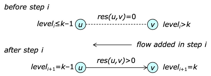
Proof. Suppose the claim is not true and that $k$ is the smallest integer for which there is some vertex $v$ with $\level_{i+1}(v)=k < \level_{i}(v)$. Let $e$ be an edge joining $u$ and $v$ with $\res_e(u,v)>0$ following step $i$ with $\level_{i+1}(u)=k-1$ and note that $\level_{i}(u)\leq k-1$.
Since $\level_{i}(v) > k$, $\res_e(u,v)=0$ before step $i$. This means that step $i$ must have added flow to the edge from $v$ to $u$. This implies that $\level_{i}(v)=\level_{i}(u)-1 \leq k-2$ contradicting the original assumption that $\level_{i}(v)>k$. This argument is summarized in the diagram below.
The next step is to show that $\level_i(t)$ increases by at least 1 after every $m$ steps.
Lemma 2. If the number of augmenting path steps is $\geq i+m$, then $\level_{i+m}(t) > \level_i(t)$.
Proof. For a path $p$ with vertices $[u_0,\ldots,u_k]$, define $\level_i(p)$ to be the vector $[\level_i(u_0),\ldots,\level_i(u_k)]$. Let $p_i$ be the augmenting path chosen in step $i$ and $p_j$ the augmenting path chosen in step $j\geq i$. If $p_i$ and $p_j$ have length $k$ then $\level_j(p_j)=[0,\ldots,k]=\level_i(p_i)$.
The lemma can be proved by showing that $\level_j(p_j)=\level_i(p_j)$. Assume that $j$ is the smallest integer for which $\level_j(p_j)\neq \level_i(p_j)$. Since $p_i$ and $p_j$ have the same length and both end at $t$, $\level_j(t)=\level_i(t)$. Let $u$ be the last vertex on $p_j$ for which $\level_j(u) \neq \level_i(u)$, and let $e$ be the edge linking $u$ to its successor $v$ on $p_j$. Since $$\level_j(u) \neq \level_i(u) = \level_{j-1}(u)$$ $\level_{j-1}(u) < \level_j(u)$ by the previous lemma. Since $\level_j(v)=\level_{j-1}(v)$, $\res_e(u,v)$ must have been zero just before step $j-1$. Since that is not true after step $j-1$, step $j-1$ must have added flow from $v$ to $u$. This implies $$\level_{j-1}(u) > \level_{j-1}(v)=\level_j(v)>\level_j(u)$$ yielding a contradiction.
Let $P$ be the set of paths $p_j$ with $j\geq i$ and $p_j$ and $p_i$ of the same length. Define two augmenting paths to be consistent if for every edge on both paths, the direction of flow is the same. Since $\level_j(p_j)=\level_i(p_j)$ for all $p_j\in P$, all pairs of paths in $P$ are consistent. Consequently, no edge used by paths in $P$ can be saturated more than once. Since every augmenting step saturates at least one edge, the number of augmenting paths in $P$ is at most $m$. Consequently, $\level_{i+m}(t) > \level_i(t)$. $\Box$
Since augmenting paths are simple and $\level_i(t) \leq n-1$, $\level_i(t)$ can increase at most $n-2$ times. By Lemma 2 it must increase by at least once every $m$ steps, so the number of steps is $\leq mn$ and the running time of the algorithm is $O(m^2n)$. The example below shows how the worst-case behavior can arise.

In this example, the first nine augmenting paths have length 11 and pass through the top left chain of vertices, the central bipartite subgraph and the bottom right chain of vertices. The next nine have length 15 and pass through the bottom left chain, back, up through the central subgraph and then through the top right chain. Subsequent groups of paths (of length 19, 23, 27 and 31) are similar, passing through the central subgraph in alternating directions. As the example is scaled up, the running time scales as $k^5$ and since $k$ is proportional to $n$, this is $\Omega(n^5)$.
Lemma 3. There is a sequence of $\leq m$ augmenting path steps that leads to a maximum flow.
Proof. Given a maximum flow on $G$, remove all edges with zero flow. Let $p$ be a path from $t$ to $s$ with positive residual capacity, $\delta$. Push $\delta$ units of flow along $p$ and remove all edges that now have zero flow. This must remove at least one edge, so repeating this process, all edges will have been deleted in at most $m$ steps. The selected paths can all be reversed, making them augmenting paths in $G$. $\Box$
Lemma 3 can be used to bound the number of steps used by the version of the augmenting path method that selects maximum residual capacity paths.
Define $\rem_i$ to be the difference between the maximum flow value and the current flow value, just before step $i$. From the argument used in the proof of Lemma 3, there is a sequence of at most $m$ augmenting steps leading to a maximum flow. Therefore, the maximum capacity path must have capacity at least $\rem_i/m$. If the total number of augmenting path steps is greater than $i+2m$, then at least one of the next $2m$ steps must add less than $\rem_i/2m$ units of flow. This means that after $2m$ steps, the capacity of the maximum capacity path is reduced by at least a factor of 2. If the maximum edge capacity is $C$, the number of augmenting path steps is $O(m\log C)$ and if $C$ is poloynomial in $n$, this is $O(m\log n)$.
One can use a variant of Dijkstra's algorithm to find paths with maximum residual capacity. As with Dijkstra's algorithm, a heap is used to keep track of vertices at the border of a tree whose paths are all maximum capacity paths. A border vertex $u$ is stored in the heap using a key matching the residual capacity of the best edge examined so far from a tree vertex to $u$. A Javascript implementation of the findpath function used by the maximum capacity augmenting path algorithm is shown below.
The running time for the max capacity algorithm is $O(m^2(\log_{2+m/n} n)(\log C))$. For dense graphs, this is $O(m^2(\log C))$ and if $C$ is polynomial in $n$, $O(m^2 \log n)$.
The following script can be used to run the program in the web app.
let g = new Flograph();
g.fromString('{a->[b:3 d:2] b[c:3 d:7 g:3] c[d:1 e:5] d[e:2 f:1 g:3] ' +
             'e[f:1 g:3 h:4] f[e:1 g:2 h:3] g[e:3 f:2 h:1] ' +
             'h[f:3 i:4 j:2] i[g:5 j:6] ->j[]}');
let [ts] = maxflowFFmc(g,1);
log(ts);
This produces the output
augmenting paths with residual capacities
a:3 b:3 c:5 e:4 h:2 j
a:2 d:2 e:2 h:4 i:6 j
a:1 b:3 g:1 h:2 i:4 j

{
a->[b:3/3 d:2/2] b[c:3/2 d:7 g:3/1] c[d:1 e:5/2]
d[e:2/2 f:1 g:3] e[f:1 g:3 h:4/4] f[e:1 g:2 h:3]
g[e:3 f:2 h:1/1] h[f:3 i:4/3 j:2/2] i[g:5 j:6/3] ->j[]
}
Note how the findpath method uses breadth-first search over the edges with residual capacity larger than the scale threshold. If it fails to find a path at the current scale value, it halves the value and tries again. Running maxflowFFcs in place of maxflowFFmc in the web app produces the same output as for the maximum capacity algorithm. In general, the scaling algorithm may use more augmenting steps, although the number remains $O(m\log C)$.
function hardTest(algo, label, g, k1, k2) {
    g.clearFlow();
    let t0 = Date.now(); let [,stats] = algo(g); let t1 = Date.now();
    let fstats = g.flowStats();
    log(`${label} k1=${k1} k2=${k2} ${t1-t0}ms ` +
        `paths=${stats.paths} ` +
        `steps/path=${~~(stats.steps/stats.paths)}`);
}
let k1=10; let k2=10; let g = maxflowHardcase(k1, k2);
hardTest(maxflowFFsp, 'FFsp', g, k1, k2);
The function maxflowHardcase produces graphs that are
similar to the example given above. Indeed, if $k_1=k_2=3$,
it produces exactly the graph shown in the example.
The two parameters allow one to separately control the number
of distinct path lengths ($k_1$) and the size of the
central subgraph ($k_2$).
The results below show the effect of increasing $k_1$ from
10 to 80, while holding $k_2$ fixed.
FFsp k1=10 k2=10   44ms paths= 2000 steps/path= 575
FFsp k1=20 k2=10  127ms paths= 4000 steps/path= 866
FFsp k1=40 k2=10  426ms paths= 8000 steps/path=1446
FFsp k1=80 k2=10 1524ms paths=16000 steps/path=2606
Note that the number of augmenting paths grows directly with $k_1$, and as the paths get longer, so does the average number of steps per path. Consequently, the running time grows quadratically. The results below show the effect of increasing $k_2$ from 10 to 80, while holding $k_1$ fixed.
FFsp k1=10 k2=10     46ms paths=  2000 steps/path=  575
FFsp k1=10 k2=20    254ms paths=  8000 steps/path= 1255
FFsp k1=10 k2=40   2491ms paths= 32000 steps/path= 3814
FFsp k1=10 k2=80  37982ms paths=128000 steps/path=13732
In this case, the number of augmenting paths grows quadratically with $k_2$ as does the number of steps per path. Consequently, the run time grows as the fourth power of $k_2$.
While these graphs are not really worst case for the max capacity and capacity scaling algorithms, it's still interesting to see how they behave.
FFmc k1=10 k2=10  1ms paths= 20 steps/path= 562
FFmc k1=20 k2=10  2ms paths= 40 steps/path= 995
FFmc k1=40 k2=10  8ms paths= 80 steps/path=1830
FFmc k1=80 k2=10 26ms paths=160 steps/path=3526

FFmc k1=10 k2=10  1ms paths= 20 steps/path= 562
FFmc k1=10 k2=20  4ms paths= 40 steps/path= 949
FFmc k1=10 k2=40 15ms paths= 80 steps/path=1638
FFmc k1=10 k2=80 41ms paths=160 steps/path=2746
For the max capacity algorithm, the number of paths grows directly with both parameters. Note that all the paths bypass the central bipartite graph, leading to a much smaller number of path searches. The average number of steps per path search also grows directly with both parameters, consequently the run time grows quadratically in both cases.
FFcs k1=20 k2=10  2ms paths= 40 steps/path= 862
FFcs k1=40 k2=10 14ms paths= 80 steps/path=1445
FFcs k1=80 k2=10 23ms paths=160 steps/path=2607

FFcs k1=10 k2=10  1ms paths= 20 steps/path=  568
FFcs k1=10 k2=20  2ms paths= 40 steps/path= 1232
FFcs k1=10 k2=40 11ms paths= 80 steps/path= 3727
FFcs k1=10 k2=80 47ms paths=160 steps/path=13397
For capacity scaling, the number of paths grows directly with $k_1$ but the number of steps per path grows quadratically with $k_2$, as most path searches must examine the edges in the central subgraph to determine that their residual capacity falls below the scale threshold. The use of the heap in the max capacity algorithm allows it to avoid examining most of these edges.
To compare the performance of the various augmenting path algorithms on random graphs, enter the following script in the web app.
function randomTest(algo, label, g, d) {
    g.clearFlow();
    let t0 = Date.now(); let [,stats] = algo(g); let t1 = Date.now();
    let fstats = g.flowStats();

    log(`${label} n=${g.n} d=${d} cutSize=${fstats.cutSize} ${t1-t0}ms ` +
        `paths=${stats.paths} steps/path=${~~(stats.steps/stats.paths)}`);
}

let n=202; let d=25;
let g = randomFlograph(n, d);
g.randomCapacities(randomInteger, 1, 99);

randomTest(maxflowFFsp, 'FFsp', g, d);
randomTest(maxflowFFmc, 'FFmc', g, d);
randomTest(maxflowFFcs, 'FFcs', g, d);
The randomFlograph() function produces a graph on $n$ vertices
with average out-degree $d$ and a built-in “small cut”.
In this case, that small cut contains 125 edges and splits the vertex
set in half. (This function can also be used to generate graphs with multiple
small cuts.)
Running the script produces the output shown below.
FFsp n=202 d=25 cutsize=125  63ms paths=331 steps/path=8176
FFmc n=202 d=25 cutsize=125 118ms paths=142 steps/path=9659
FFcs n=202 d=25 cutsize=125  36ms paths=217 steps/path=7372
The shortest path variant requires more path searches, as expected. Still, the difference in running time is less than a factor of two. Doubling the number of vertices produces the following results.
FFsp n=402 d=25 cutsize=138 160ms paths=380 steps/path=18075
FFmc n=402 d=25 cutsize=138 423ms paths=163 steps/path=21937
FFcs n=402 d=25 cutsize=138  88ms paths=236 steps/path=15452
Doubling the average vertex degree (and hence the number of edges) produces the results below.
FFsp n=402 d=50 cutsize=500 1111ms paths=1202 steps/path=35208
FFmc n=402 d=50 cutsize=500 1358ms paths= 551 steps/path=29553
FFcs n=402 d=50 cutsize=500  595ms paths= 761 steps/path=30032
Notice the large increase in the size of the small cut in this case. This contributes to an increase in the number of path searches by all three algorithms that is roughly proportional to the increase in cut size. The number of steps per path also goes up substantially for all three.
At the start of each phase, Dinic's algorithm computes a function $\level(u)$, which is the length of a shortest path with positive residual capacity from $s$ to $u$. During the phase, path searches are restricted to edges $e$ joining vertices $u$ and $v$ with $\res_e(u,v)>0$ and $\level(v) = \level(u)+1$ and $\level(u)< \level(t)$.
The resulting “searchable subgraph” can be viewed as a directed acyclic graph. Path searches are done using depth-first search in this graph, with paths leading to dead-ends being effectively “pruned”, making later searches more efficient. A Javascript implementation of Dinic's algorithm appears below.
The findpath function uses depth-first search, returning true whenever it finds an augmenting path and false, otherwise. Note that $\textit{nextedge}[u]$ specifies the next edge to be processed at u within a phase. It is intialized to the first vertex on $u$'s adjacency list at the start of the phase and is advanced to the next vertex on the list whenever the search determines that the current nextedge value leads to a dead end.
From the earlier analysis of the shortest augmenting path algorithm, the value of $\level(t)$ increases with each phase of Dinic's algorithm, which means the number of phases is $< n$. The computation of $\level$ at the start of each phase takes $O(m)$ time and the number of path searches per phase is at most $m$. To determine the number of steps required for the path searches, let $N_i$ be the number of edges examined by the $i$-th top-level call to findpath and note that the time required for all calls to findpath is $O(\sum N_i)$. The nextedge pointer is advanced to the next edge for every edge examined that is not part of the path returned by findpath. Since the path length is at most $n$, pointers are advanced at least $N_i-n$ times during the $i$-th call to findpath. But during the phase, the nextedge pointers can be advanced at most $2m$ time, so $\sum_{1\leq i\leq m} (N_i-n) \leq 2m$ and $\sum N_i = O(mn)$. Thus, the overall running time is $O(mn^2)$
The worst-case example shown earlier for the shortest augmenting path
algorithm is also a worst-case for Dinic's algorithm. It does end up
being substantially faster on this example because it avoids re-examining
the entire central subgraph on each path search.
Note that it does still trace the long chains of vertices leading
to and from the central subgraph on each path search.
The time spent following those chains can be significantly reduced
using the dynamic trees data structure of Sleator and Tarjan.
Using Dynamic Trees to Represent Unsaturated Paths
The dynamic trees
data structure can be used to speed up
augmenting path searches, by storing information about previously
explored paths with positive residual capacity.
Each vertex $u$ with parent $v$ in the dynamic trees data
structure is associated with an edge $e$ joining $u$ and $v$ in the
flow graph with $\res_e(u,v)>0$ and $\level(v)=\level(u)+1$.
The cost of $u$ in the dynamic trees
data structure is set to $\res_e(u,v)$, while the cost of every root
vertex is set to a value large enough so that the root is never the
minimum cost node on a tree path.
Consequently, the path from $u$ to its tree root corresponds to
an unsaturated path in the flow graph and the residual capacity of
this path is the minimum cost of any vertex on the tree path.
For flow graph edges that are not associated
with a tree edge, flow information is maintained in the flow graph.
The figure illustrates the use of dynamic trees. It shows two trees overlaid on the edges of a flow graph joining vertices $u$ and $v$ for which $\level(v)=\level(u)+1$. Note that the minimum cost on the tree path from $a$ to $i$ is 3, implying that the residual capacity of the path in the flow graph is also 3. Subtracting 3 from the cost of this tree path effectively adds 3 units of flow to all the edges on the path in the flow graph.
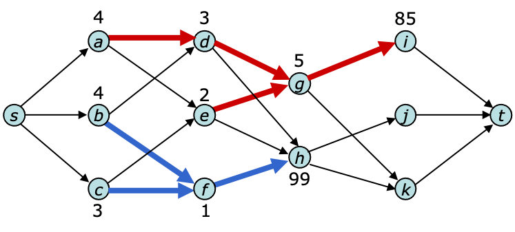
The findpath function uses the dynamic trees data structure to take shortcuts through the flow graph, linking trees together until there is a tree path from the source to the sink. When dead ends are discovered, they are pruned from the tree. Because the average time per operation in a sequence of dynamic tree operations is $O(\log n)$, this reduces the worst-case bound for each phase of the algorithm by a factor of $n/\log n$.
A Javascript implementation of the dynamic trees variant of Dinic's algorithm is shown below.
The first of the two inner loops in the findpath method combines trees in the dynamic trees data structure in order to create a tree path from the source to the sink. The extend method makes the required changes to the tree and sets the cost to reflect the residual capacity. If it fails to extend the tree containing the source vertex at some point, the loop terminates and the second of the two inner loops is executed. This loop prunes the dead end encountered in the first loop. This involves removing all the tree edges entering the dead end vertex and transferring the flow information for these tree edges to the corresponding flow graph edges. The prune method handles these details.
During one phase, prune is called at most $m$ times. To see this, note that whenever it is called from findpath or augment, one of the nextEdge pointers is advanced. The number of calls to extend is also at most $m$ since no edge is added to the dynamic trees data structure more than once. This means that there are $O(m)$ operations performed on the dynamic trees data structure during a phase and that the running time contributed by these operations is $O(m\log n)$, and so the overall runnning time is $O(mn\log n)$.
let k1=10; let k2=10; let g = maxflowHardcase(k1, k2);

hardTest(maxflowFFsp, 'FFsp', g, k1, k2);
hardTest(maxflowD,    'D   ', g, k1, k2);
hardTest(maxflowDST,  'DST ', g, k1, k2);
Running this for three parameter settings produces the results below.
n=456 m=1225
FFsp k1=25 k2=25  1889ms paths= 31250 steps/path=2181
D    k1=25 k2=25   135ms paths= 31250 steps/path= 334
DST  k1=25 k2=25   232ms paths= 31250 steps/path=  32
n=906 m=3700
FFsp k1=50 k2=50 46182ms paths=250000 steps/path=6856
D    k1=50 k2=50  2087ms paths=250000 steps/path= 632
DST  k1=50 k2=50  1621ms paths=250000 steps/path=  28
In the second group, the number of paths goes up by a factor of eight, so the number of steps per path is the key metric. For the shortest augmenting path algorithm this goes up roughly in proportion to the number of edges. For Dinic's algorithm it goes up roughly in proportion to the number of vertices. For the version using dynamic trees it actually comes down as the number of paths per phase grows. So both versions of Dinic's algorithm are dramatically faster than the shortest augmenting paths algorithm. The higher overhead of the dynamic trees variant makes it slower for the smaller graphs.
To compare the algorithms on random graphs, enter the following script in the web app.
let n=202; let d=25;
let g = randomFlograph(n, d);
g.randomCapacities(randomInteger, 1, 99);

randomTest(maxflowFFsp, 'FFsp', g, d);
randomTest(maxflowD,    'D   ', g, d);
randomTest(maxflowDST,  'DST ', g, d);
Here are the results from running this with three parameter settings.
FFsp n=202 d=25 cutsize=125   58ms paths= 287 steps/path=8507
D    n=202 d=25 cutsize=125    2ms paths= 287 steps/path= 370
DST  n=202 d=25 cutsize=125    9ms paths= 287 steps/path= 542

FFsp n=402 d=25 cutsize=138  148ms paths= 357 steps/path=17755
D    n=402 d=25 cutsize=138    6ms paths= 357 steps/path=  599
DST  n=402 d=25 cutsize=138   18ms paths= 357 steps/path=  885

FFsp n=402 d=50 cutsize=500 1006ms paths=1178 steps/path=34114
D    n=402 d=50 cutsize=500   11ms paths=1178 steps/path=  305
DST  n=402 d=50 cutsize=500   28ms paths=1178 steps/path=  439
Once again, both versions of Dinic's algorithm are dramatically faster, due to the more efficient path searches, but the version using dynamic trees is actually slower than the standard version. This can be explained by the shorter augmenting path lengths in the random graphs and the much more limited opportunity to exploit shortcuts. Indeed, the contrast between the random and hard test cases makes it clear that the dynamic trees data structure is really only likely to be advantageous in artificial situations where long path segments show up in large numbers of augmenting paths. It's unlikely that this will happen much in practice, making the practical benefit of dynamic trees somewhat questionable. On the other hand, it is never dramatically slower than the simpler version, and it may occasionally be significantly faster.
Select an unbalanced vertex $u$; if $u$ has an admissible edge $e=(u,v)$, add $\min\{\res_e(u,v), \Delta(u)\}$ units of flow from $u$ to $v$; otherwise, expand the set of admissible edges at $u$.
So, the preflow-push method attempts to balance vertices by pushing flow out on its admissible edges. Goldman and Tarjan [GT86] proposed a method for determining which edges should be admissible that is similar to the level function in Dinic's algorithm. Each vertex $u$ is assigned a distance label $d(u)$ and an edge $e=(u,v)$ is defined to be admissible at $u$ if $\res_e(u,v)>0$ and $d(u)=d(v)+1$. The distance labels are said to be valid if $d(s)=n$, $d(t)=0$ and $d(u)\leq d(v)+1$ for every edge $e=(u,v)$ with $\res_e(u,v)>0$. Distance labels are said to be exact if $d(u)= d(v)+1$ for every edge with $\res_e(u,v)>0$.
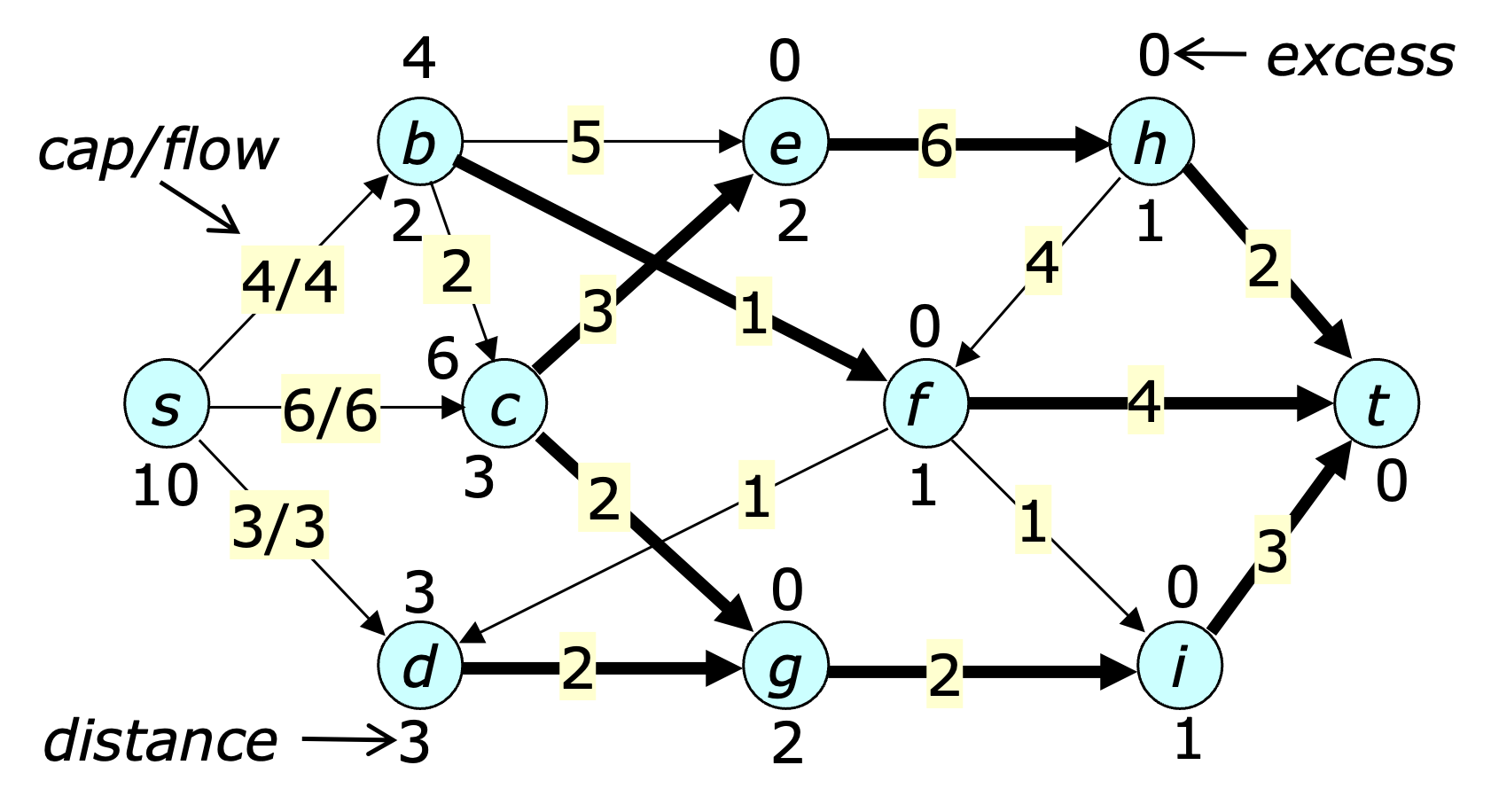
With these definitions, the general preflow-push method can be stated as follows. Saturate all edges leaving the source and initialize the distance labels by setting $d(s)=n$ and $d(u)$ to the length of the shortest unsaturated path from $u$ to the sink, for all other vertices. Then, repeat the following step, so long as there is an unbalanced vertex.
Select an unbalanced vertex $u$; if $u$ has an admissible edge $e=(u,v)$, add $\min\{\res_e(u,v), \Delta(u)\}$ units of flow from $u$ to $v$; otherwise, let $d(u)=\min_v d(v)+1$ where the minimum is over all neighboring vertices $v$ with $\res(u,v)>0$.
Note that each step preserves the validity of the distance labels. Following initialization, there is a saturated cut separating the source from the sink. This remains true at every step. To understand why, note that if a saturated cut exists before a step at vertex $u$ but not after the step, the step must add flow to an edge $e=(u,v)$ and this edge must be in such a cut. Also, adding flow to the edge must create an augmenting path and that path must pass from vertex $v$ through edge $e$ to $u$. However, since the step adds flow from $u$ to $v$, there must be an unsaturated path from $v$ to $t$ before the step and this implies that there was also an augmenting path from $s$ to $t$ before the step. Since there is still a saturated cut when the method terminates, the flow at that point must be a maximum flow.
The figure below shows a flow graph just after the preflow-push initialization. The excess flow at each vertex is shown above the vertex, while the distance label is shown below it. The admissible edges are highlighted in bold.
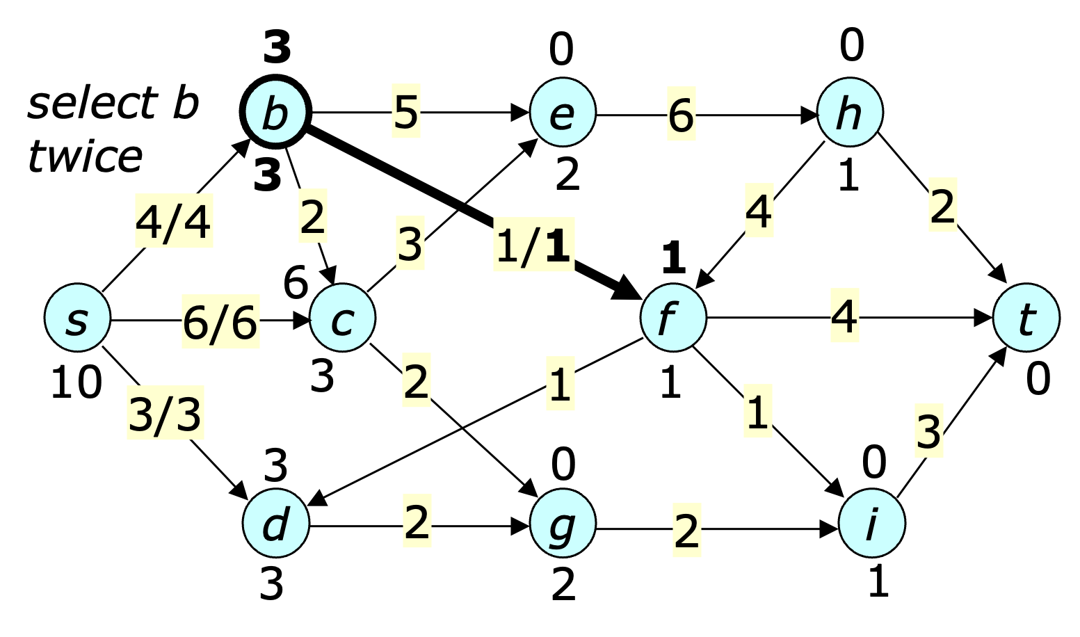
The figure below shows the state of the flow graph after $b$ is selected two times. In this case, the bold highlighting is used to emphasize what has changed. Note that at this point, the edge $(b,e)$ is admissible at $b$.
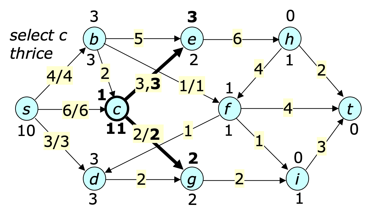
The next figure shows the state after $c$ is selected three times.
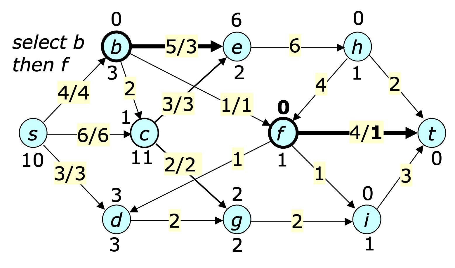
The next step shows the state after $b$ is selected once followed by $f$. Note that both vertices are now balanced.
Continuing in this fashion, eventually leads to a situation where all vertices are balanced. Note that the basic version of the preflow-push method does not specify which vertex to select at each step. Specific selection methods can make the method more efficient. Still, it's worthwhile analyzing the performance of the general method, since portions of the analysis carry over to the more efficient variants.
First, note that every unbalanced vertex $u$ has an unsaturated path back to the source throughout the execution of the method. This follows easily by induction on the number of steps. Next, note that whenever a vertex $u$ is relabeled, it is unbalanced, and so the existence of an unsaturated path to the source plus the validity of the distance labels implies that $d(u) <2n$. This implies that the each vertex is relabled $<2n$ times, since each step increases the label by at least 1. The time required to relabel a vertex is bounded by the number of edges incident it, so the total time spent relabeling all vertices is $O(mn)$.
As long as the label of a vertex does not change, none of its non-admissible edges can become admissible. This means that once an edge at $u$ has been checked for admissibility, it need not be checked again until $u$ is relabeled. If $\nextedge(u)$ is initialized to the first edge in $u$'s adjacency list whenever $u$ is relabeled and is advanced to the next edge in the adjacency list whenever an inadmissible edge is found, all edges at $u$ can be checked for admissibility in a single pass through the adjacency list for each relabeling of $u$. Since each vertex is relabeled $<2n$ times, the total time spent searching for admissible edges is $O(mn)$.
Since any step that saturates an edge $e=(u,v)$ makes $e$ inadmissible at $u$ and because fewer than $2n$ steps make any edge admissible at $u$, the time spent on steps that saturate an edge at $u$ is $O(mn)$. What remains is to determine the time spent on steps that add flow to an edge but do not saturate it. The following lemma bounds the number of these steps.
Lemma 4. The number of steps that add flow and do not saturate an edges is $O(mn^2)$.
Proof. The total number of steps taken be the algorithm can be bounded using an amortized complexity analysis that uses the following credit policy.
The number of credits on hand is always at least equal to the sum of the distance labels at the unbalanced vertices.
The policy can be satisfied at the start of execution using fewer than $2n^2$ credits and each step may require additional credits to satisfy the credit policy and account for the step. There are three cases.
Because each step that adds flow to an edge without saturating it takes constant time (excluding the time spent identifying admissible edges), the time spent on these steps is $O(mn^2)$ as is the overall runnning time of the algorithm. Thus, the general preflow-push method has the same worst-case performance as Dinic's algorithm.
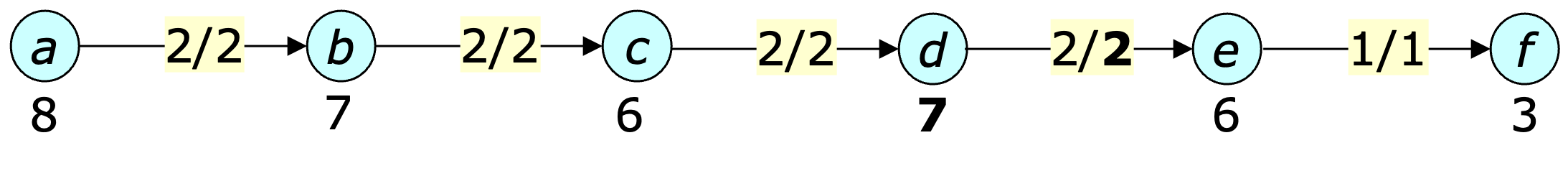
The preflow-push does have one drawback that any actual implementation needs to address in order to get good performance in practice. Specifically, it can spend a lot of time pushing excess flow out back out of portions of the graph with no remaining unsaturated paths to the sink. A simple example of this is shown below.

Note that $e$ is unbalanced, so if $e$ is selected next, it will be relabeled, allowing flow to be pushed back to $d$ on the next step.

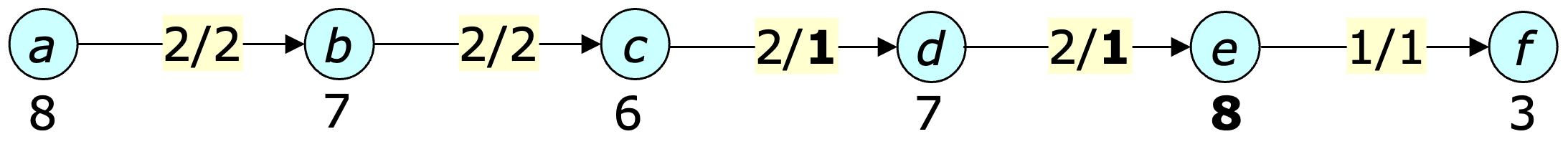
At this point, $d$ is unbalanced and if it is selected next, it will be relabeled allowing flow to be pushed forward to $e$ again.
Since $e$ is now unbalanced, it can be relabeled and flow pushed back to $d$ and $c$ in the next two steps.
At this point $c$ is relabeled, allowing flow to move forward again to $d$, which is then relabeled and sends flow forward to $e$. This pattern of back and forth flow adjustments continues until the labels at vertices $b$ through $e$ increase to 9, 10, 11 and 12. For longer paths, the number of steps grows quadratically with the path length. Clearly, there is a lot of wasted effort here. The source of this inefficiency is the incremental adjustment of distance labels.
It's instructive to compare the incremental adjustment of vertex labels to the periodic recomputation of the level function in Dinic's algorithm. That approach can also be incorporated into the preflow-push method. Specifically, the relabelling can be deferred until all unbalanced vertices are processed. At that point, if there are still unbalanced vertices, exact vertex labels are computed for all vertices. This “batch relabel” approach is usually significantly faster than incremental relabeling, although they both share the same worst-case performance. It turns out that an intermediate approach that alternates between incremental relabeling and batch relabeling can be even more efficient. There are several strategies one can use to implement such an approach. One such strategy is used in the Javascript implementation described in the next section.
The performance of the FIFO variant can be analyzed by dividing the execution into phases. A phase ends when all vertices on the queue at the start of the phase have been selected. Each phase contains at most $n$ steps that add flow to an edge without saturating it (since each such step balances a vertex), so if the number of phases is $O(n^2)$, the overall running time is $O(n^3)$.
Since the number of steps that relabel a vertex is $<2n^2$, the number of phases that include at least one such step is also $<2n^2$. An amortized analysis can be used to bound the number of phases that do not include a step that relabels a vertex. The required credit policy is stated below.
The number of credits on hand is never less than the largest label at an unbalanced vertex.
The policy can be satisfied initially using $<2n$ credits. In every phase in which no vertex is relabeled, every vertex that was unbalanced at the start of the phase becomes balanced. Since each step pushes flow to vertices with smaller labels, The largest label at an unbalanced vertex must decrease by at least 1 during such a phase, reducing the number of credits needed to satisfy the credit policy and providing a credit that can be used to account for the phase.
The phases that do relabel vertices may increase the number of required credits, since each increase in a label has the potential to increase the maximum label. Since the total increase in the labels over the course of the algorithm is $<2n^2$, the number of credits that must be allocated for these phases is $O(n^2)$. Consequently, the total number of credits allocated is $O(n^2)$ and the number of phases in which no vertex is relabeled is also $O(n^2)$.
The Javascript implementation of the preflow-push method is divided into parts. There is a core module that implements the portion of the algorithm that is common to all variants, and for each variant, there is another module that handles the processing that is specific to that variant. The module for the FIFO variant appears below.
The function putUnbal adds a vertex to the set of unbalanced vertices and the function getUnbal removes a vertex from the unbalanced set and returns it. These functions are passed to the core module, which calls them as needed. The core module is shown below.
The balance() function attempts to balance flow at a vertex by pushing flow out on its admissible edges. It returns when it has balanced the vertex or examined all of its admissible edges.
Observe that when the program is operating in batch mode, it simply attempts to balance all the unbalanced vertices, without doing any incremental relabeling operations. When not in batch mode, each unsuccessful balance attempt causes a vertex to be relabeled.
The optional parameter relabThresh determines when the program switches from incremental relabeling to batch relabeling. The incrRelabelSteps counter is incremented for each edge examined by the minlabel method. Whenever batch relabeling is performed, incremental relabeling is enabled until the number of additional computational steps performed by the incremental relabeling code exceeds relabThresh. At that point, the program switches to batch mode, suspending incremental relabeling until all unbalanced vertices have been processed and another batch relabeling has been performed. Note that the default value for relabThresh is $g.m$. This choice ensures that the total amount of computation done for incremental relabeling roughly matches that for batch relabeling.
The following script can be used to demonstrate the FIFO method.
let g = new Flograph();
g.fromString('{a->[b:5 d:6] b[c:3 d:7 g:3] c[d:1 e:5] d[e:2 f:1 g:3] ' +
             'e[f:1 g:3 h:4] f[e:1 g:2 h:3] g[e:3 f:2 h:1] ' +
             'h[f:3 i:4 j:5] i[g:5 j:6] ->j[]}');
let [ts] = maxflowPPf(g,g.m,1);
log(ts);
Running this produces the trace output shown below.
Each line shows the relabeling mode ('B' for batch, 'I' for incremental),
the selected unbalanced vertex,
its distance label and excess flow, followed by the
number of incremental relabeling steps since the last
batch relabeling and the edges
on which flow was pushed during the balancing operation.
A single asterisk at the end of a line indicates that an
incremental relabeling operation was done at that point,
and a double asterisk indicates that a batch relabeling
was done. The final flow is shown at the end.
mode, unbalanced vertex, distance label, excess, relabel steps, push edges
I d 3 6 0 (d,e,2/2) (d,f,1/1) (d,g,3/3)
I b 3 5 0 (b,g,3/3) *
I e 2 2 4 (e,h,4/2)
I f 2 1 4 (f,h,3/1)
I g 2 6 4 (g,h,1/1) *
I b 4 2 12 (b,c,3/2)
I h 1 4 12 (h,j,5/4)
I g 3 5 12 (g,e,3/3) (g,f,2/2)
I c 3 2 12 (c,e,5/2)
I e 2 5 12 (e,h,4/4) *
I f 2 2 19 (f,h,3/3)
I h 1 4 19 (h,j,5/5) *
B e 3 3 25 (e,f,1/1)
B h 2 3 25 (h,i,4/3)
B f 2 1 25
B i 1 3 25 (i,j,6/3) **
I e 12 2 0 (d,e,2)
I f 12 1 0 (d,f,1)
I d 11 3 0 (a,d,6/3)

{
a->[b:5/5 d:6/3] b[c:3/2 d:7 g:3/3] c[d:1 e:5/2]
d[e:2 f:1 g:3/3] e[f:1/1 g:3 h:4/4] f[e:1 g:2 h:3/3]
g[e:3/3 f:2/2 h:1/1] h[f:3 i:4/3 j:5/5] i[g:5 j:6/3] ->j
}
A Javascript implementation of this version of the preflow-push method appears below.
Observe that a singe call to the getUnbal function can require up to $2n$ iterations of the while loop. However, the total number of iterations over all calls can be bounded by the total increase in the distance labels. This implies that the total time spent in the while loop is $O(n^2)$.
The trace output from maxflowPPhl when run on the sample graph from the last section is shown below.
mode, unbalanced vertex, distance label, excess, relabel steps, push edges
I d 3 6 0 (d,e,2/2) (d,f,1/1) (d,g,3/3)
I b 3 5 0 (b,g,3/3) *
I b 4 2 4 (b,c,3/2)
I c 3 2 4 (c,e,5/2)
I e 2 4 4 (e,h,4/4)
I f 2 1 4 (f,h,3/1)
I g 2 6 4 (g,h,1/1) *
I g 3 5 12 (g,e,3/3) (g,f,2/2)
I e 2 3 12 *
I e 3 3 19 (e,f,1/1) *
B e 4 2 26 (g,e,3/1)
B g 3 2 26
B f 2 3 26 (f,h,3/3)
B h 1 8 26 (h,j,5/5) **
I g 12 2 0 (d,g,3/1)
I f 12 1 0 (d,f,1)
I d 11 3 0 (a,d,6/3)
I h 2 3 0 (h,i,4/3)
I i 1 3 0 (i,j,6/3)

{
a->[b:5/5 d:6/3] b[c:3/2 d:7 g:3/3] c[d:1 e:5/2]
d[e:2/2 f:1 g:3/1] e[f:1/1 g:3 h:4/4] f[e:1 g:2 h:3/3]
g[e:3/1 f:2/2 h:1/1] h[f:3 i:4/3 j:5/5] i[g:5 j:6/3] ->j
}
The first line below shows results for the pure batch relabeling approach, the last line shows the pure incremental approach and the middle line shows the mixed approach using the default value of relabThresh. Note that each batch relabeling operation contributes $2m$ relabeling steps.
PPf n=1002 d=25  21ms rcount=   11 rsteps= 550550 bcount= 2249 bsteps=  86598
PPf n=1002 d=25  10ms rcount=  924 rsteps= 206187 bcount= 3338 bsteps= 118603
PPf n=1002 d=25 144ms rcount=40263 rsteps=2609132 bcount=71892 bsteps=2578176
The number of relabel steps and balance steps is much higher for the pure incremental approach, due to the large number of mostly unproductive incremental relabeling steps that occur towards the end of execution, as flow is pushed back towards the source. Because each batch relabeling operation is relatively expensive, a mixed approach works better than a pure batch approach. Even a fairly small value of the relabeling threshold yields some improvement, but the default value effectively balances the computation from incremental relabeling steps with those from batch relabeling steps.
The results below compare the FIFO and highest-label-first approaches for three different random graphs.
PPf  n=1002 d=25 10ms rcount= 954 rsteps= 207659 bcount= 3395 bsteps=121641
PPhl n=1002 d=25 11ms rcount= 923 rsteps= 207196 bcount= 3934 bsteps=113743

PPf  n=2002 d=25 21ms rcount=1751 rsteps= 407780 bcount= 5591 bsteps=214861
PPhl n=2002 d=25 22ms rcount=1810 rsteps= 413090 bcount= 6924 bsteps=209169

PPf  n=2002 d=50 48ms rcount=1905 rsteps= 828952 bcount= 6632 bsteps=494245
PPhl n=2002 d=50 59ms rcount=2613 rsteps=1123705 bcount=10136 bsteps=628053
The FIFO method out-performs the highest label first method and this pattern generally holds up for larger and more sparse random graphs as well. However, the highest label method can perform better for the worst-case graphs for Dinic's algorithm.
n=456 m=1225
PPf  k1=25 k2=25  6ms rcount= 3772 rsteps= 47457 bcount=15886 bsteps= 36612
PPhl k1=25 k2=25  5ms rcount= 3584 rsteps= 43439 bcount=11638 bsteps= 28331
n=906 m=3700
PPf  k1=50 k2=50 23ms rcount=17567 rsteps=233153 bcount=80417 bsteps=182712
PPhl k1=50 k2=50 18ms rcount=16042 rsteps=155223 bcount=49396 bsteps= 98281
Both perform much better than either version of Dinic's algorithm, as can be seen from the earlier results reproduced below.
n=456 m=1225
D    k1=25 k2=25  135ms paths= 31250 steps/path=334
DST  k1=25 k2=25  232ms paths= 31250 steps/path= 32
n=906 m=3700
D    k1=50 k2=50 2087ms paths=250000 steps/path=632
DST  k1=50 k2=50 1621ms paths=250000 steps/path= 28
For random graphs, the advantage over Dinic's algorithm is smaller, but still significant.

If the maximum flow does not saturate all edges from $s'$, there is no flow that is compatible with the specified floors. If the computed flow does saturate all edges from $s'$, each edge flow in the original graph is set to equal the computed flow for that edge plus its floor value. This is a feasible flow on the original graph for the specified floors. The feasible flow can be extended to a maximum flow, using a slightly modified definition of the residual capacity. Specifically, for an edge $e=(u,v)$, $\res_e(v,u)=f_e(u,v) - floor(e)$. This prevents the max flow algorithm from reducing the flow on an edge below its floor value.
The flow graph data structure can be extended to support flow floors using the method addFloors or by setting a floor value using setFloor. In a graph that has not been extended to support floors, the method $\textit{floor}(e)$ returns 0 for all edges. The Javascript function $\textit{flowfloor}()$ shown below, attempts to find a feasible flow for a flow graph with specified floor values.
The following script can be used to demonstrate the program. Flow floors are shown by replacing edge capacities with flow ranges. So, in the example below, the edge $(b,d)$ has a flow range of between 2 and 7, corresponding to a floor of 2.
let g = new Flograph();
g.fromString('{a->[b:3 d:2] b[c:3 d:2-7 g:3] c[d:1 e:5] d[e:2 f:1 g:3] ' +
             'e[f:1 g:3 h:1-4] f[e:1 g:2 h:3] g[e:3 f:2-7 h:1] ' +
             'h[f:3 i:4 j:2] i[g:2-5 j:6] ->j[]}');
let [,ts] = flowfloor(g, true);
log(ts);
This produces the output shown below.
flow on constructed flow graph
{
a[b:3/2 d:2] b[c:3 d:5 g:3 l:2/2] c[d:1 e:5] d[e:2/2 f:1 g:3]
e[f:1 g:3 h:3/1 l:1/1] f[e:1 g:2 h:3/2] g[e:3 f:5 h:1 l:2/2]
h[f:3 i:4/3 j:2/1] i[g:3 j:6/1 l:2/2]
j[a:75/2] k->[d:2/2 h:1/1 f:2/2 g:2/2] ->l
}
computed flow in original graph
{
a->[b:3/2 d:2] b[c:3 d:2-7/2 g:3] c[d:1 e:5] d[e:2/2 f:1 g:3]
e[f:1 g:3 h:1-4/2] f[e:1 g:2 h:3/2] g[e:3 f:2-7/2 h:1]
h[f:3 i:4/3 j:2/1] i[g:2-5/2 j:6/1] ->j
}