
The group heap implements a collection of items that are divided into groups. Each item has a key and each group may be either active or inactive. Items within active groups are also called active. Certain operations treat the collection of active items like a heap. For example, there is a $\findmin$ operation that returns the active item with the smallest key value. Each group defines an ordering over the items within it and items may be inserted into a group at a specified position within this ordering. The data structure defines the following methods.
The group heap can be implemented using an array heap $A$ to keep track of the active groups and an $\OrderedHeaps$data structure to keep track of the items within each group. The key of an active group $g$ in $A$ is the smallest key value assigned to any of the items in $g$.
The $\findmin$ operation for the group heap can be implemented by first finding the active group $g_0$ with the smallest key in $A$, then finding the item with the smallest key within $g_0$. The $\addtokeys(\Delta)$ operation can be implemented using the $\addtokeys$ operation of $A$.
Activating a group $g$ is accomplished by inserting $g$ into $A$. Deactivation removes the specified group from $A$. Note that both $A$ and the heaps for the individual groups have offsets that are used to implement $\addtokeys$. The figure below shows a group heap with two active groups, $x$ and $y$ and a single inactive group $z$.
Note that while the stored key value for $b$ is 1, the “true” value is 4. This is the value stored in $A$ for group $y$. A $\findmin$ operation on this group heap will return $c$, after using $A$ to identify group $x$ and then $x$'s heap to identify $c$.
Changes to $A$'s offset must be reflected in the offsets of the active groups, but not the inactive groups. So, before an operation is performed on an active group $g$, changes to $A$'s offset that have occurred since the most recent operation affecting $g$ are propagated to $g$'s offset. After the offset for $g$ is updated, the value of $A$'s offset is saved, to enable the next update to $g$'s offset. This process is illustrated below.

The core of the Javascript implementation is shown below.
The following script can be used to demonstrate the group heap in the web app.
let gh = new GroupHeap();
gh.fromString('{1[a:3 b:2] 2@![c:2 d:5 e:1 j:7] 6[f:6 g:3] 4@[i:10]}');
log(gh.toString());
gh.activate(1);
log(gh.toString());
log(gh.x2s(gh.findmin()));
gh.delete(5,2);
log(gh.toString());
gh.delete(3,2);
log(gh.toString());
log(gh.toString(2));
This produces the output shown below.
{1[a:3 b:2] 2@![c:2 d:5 e:1 j:7] 4@[i:10] 6[f:6 g:3]}
{1@[a:3 b:2] 2@![c:2 d:5 e:1 j:7] 4@[i:10] 6[f:6 g:3]}
e
{1@[a:3 b:2] 2@![c:2 d:5 j:7] 4@[i:10] 6[f:6 g:3]}
{1@![a:3 b:2] 2@[d:5 j:7] 4@[i:10] 6[f:6 g:3]}
[a:3 b:2 d:5 j:7 i:10]
By default, the state of the data structure is shown as a collection of
groups, with each group preceded by its group number and
each item shown with its key.
Active groups are marked with an at symbol “@”
and the active group containing the smallest key is
also marked with a exclamation point “!”.
The last line shows a more concise representation in which the
groups are hidden and only the active items are shown.

In the maximum flow problem, the dynamic trees data structure is used to represent information about edges in the graph that can accommodate more flow. Specifically, an edge linking a node $u$ to its parent represents an edge in the “flow graph” on which flow can be added. The amount of flow that can be added to that edge is represented by the cost of $u$. So any path from a node to one of its ancestors represents a path in the flow graph along which flow may be added, with the amount of flow represented by the minimum cost of the nodes along the path.
To enable efficient operations on paths in a dynamic tree, there is a special operation called $\expose$ that isolates a particular path from the rest of a tree. In fact, the tree is represented as a collection of such paths, that are linked together. The example below shows a tree that is represented in this way and the effect of an expose operation on that tree.

In the diagram, the solid edges define component paths of the tree and the dashed edges represent links joining paths together. A mapping $\succ$ maps a component path $p$ to its successor node $\succ(p)$. So for example, in the diagram, if $p$ is the path containing $m$, then $\succ(p)=n$. Note that a node can have at most one “solid edge” joining it to a child and that $\expose(u)$ turns all the dashed edges on the path from $u$ to the root into solid edges, and all solid edges incident to, but not on the path, into dashed edges.
The “solid paths” in the dynamic trees data structure are defined using another data structure called a path set. It supports the following methods.

The path sets data structure can be implemented in a way that allows $m$ operations to be completed in $O(m \log n)$ time. Details appear below. For now, let's focus on how it can be used to implement the dynamic tree operations.
The operation $\findroot(u)$ can be implemented by first doing an expose at $u$ then a $\findtail$ operation on the resulting path. Similarly, $\findcost(u)$ (and $\addcost(u)$) can be implemented by first doing an expose at $u$ and then a findpathcost (addpathcost). The operation $\graft(t,u)$ is done by first doing an expose at $t$, isolating it from the rest of its path, then a second expose at $u$, isolating the path from $u$ to its tree root, then a join adding $t$ to that path. The operation $\prune(u)$ is done by doing a $\split$ on the path containing $u$ and updating successors to account for the new path components created by the $\split$.
The expose operation is the key to the dynamic trees data structure. The diagram below illustrates how it works.
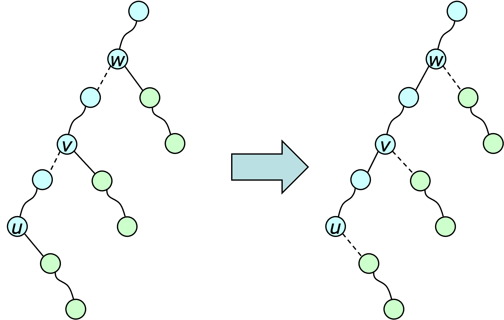
An $\expose(u)$ operation proceeds up the path from $u$ to the root, converting dashed edges along the path into solid edges and solid edges incident to the path into dashed edges. In each step, one solid path that shares part of the root path is split, and then the upper part of that path is joined to the solid path containing $u$. The successors are updated as needed to maintain the overall tree structure. So in the first step of the above example, the solid path containing $u$ is split to separate out the portion that comes before $u$. Then, $u$ is rejoined to the upper part of the path. In the second step, the solid path containing $v$ is split, then the upper part of that path is joined with the solid path containing $u$. This effectively converts a solid edge incident to the path into a dashed edge and a dashed edge on the path into a solid one. The process continues in this way until it reaches the root.
A Javascript implementation of the core methods of the dynamic trees data structure appears below.
The following script can be used to demonstrate the data structure in the web app.
let dt = new DynamicTrees();
dt.fromString('{[c:4(f:2(a:5 b:1))] [e:4(g:3(d:2 i:3(h:2)))]}');
log(dt.toString());
dt.expose(1); dt.expose(4);
log(dt.toString(0x12));
dt.graft(3,9);
log(dt.toString(0x12));
This produces the output shown below.
{[c:4(f:2(a:5 b:1))] [e:4(g:3(d:2 i:3(h:2)))]}
{f[b:1] [a:5 f:2 *c:4] [d:2 g:3 *e:4] i[h:2] g[i:3]}
{f[b:1] [*c:4 i:3 g:3 e:4] g[d:2] c[a:5 *f:2] i[h:2]}
The first line shows a pair of trees in a concise format,
with each node followed by a parenthesized list of its children.
The remaining lines show each tree as a linked collection of paths,
where an asterisk marks the node used to identify each path
and each path is preceded by its successor in its larger tree.
So in the last line, the path $[a f]$ identified by $f$ has $c$
as its successor.
In order to implement $\addpathcost$ efficiently, in the context of joins and splits, a differential representation of the node costs is used. This representation uses two mappings, $\dcost$ and $\dmin$. For each vertex $u$, if $\mincost(u)$ is the minimum cost for all nodes in $u$'s subtree, then $\dcost(u)=\cost(u) - \mincost(u)$ and $\dmin(u) = \mincost(u)$ if $u$ is a root node and $\mincost(u) - \mincost(p(u))$ if it is not. With these definitions, $\mincost(u)$ can be computed by summing the $\dmin$ fields on the path from $u$ to the root of its tree and $\cost(u)$ can be computed by adding $\dcost(u)$ to $\mincost(u)$.
Using the differential cost representation, the operation $\addpathcost(u, c)$ can be implemented by adding $c$ to $\dmin(u)$. The operation $\findpathcost(p)$ can be done by searching the tree, guided by the $\dmin$ and $\dcost$ values. Specifically, if the right child $r$ of the current node $u$ has $\dmin(r)=0$, then the target node is in the right subtree; if $\dmin(r)\neq 0$, and $\dcost(u)=0$, then $u$ is the target node; otherwise, the target is in the left subtree.
The $\join$ and $\split$ operations must update both fields at the root and its two children. The rotations used by the splays must also update the $\dmin$ and $\dcost$ values. An example of this is shown below.
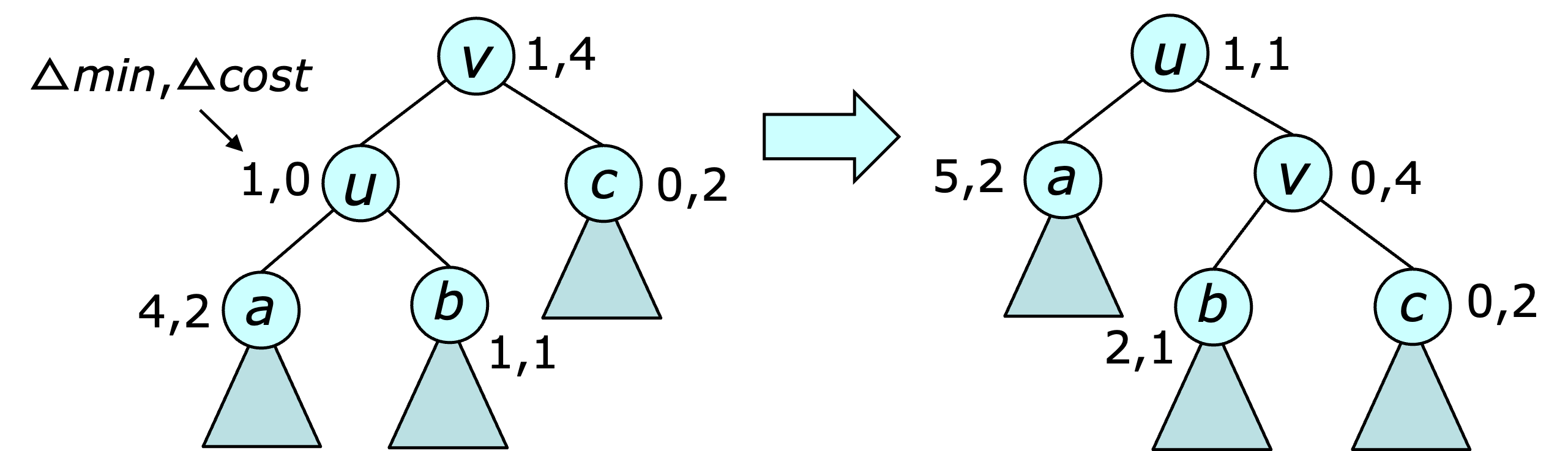
In general, the costs can be updated using the equations below. \begin{eqnarray*} \dcost\,'(u) &=& \dcost(u) + \dmin(u) \\ \dcost\,'(v) &=& \dcost(v) - \dmin'(v) \\ \dmin'(u) &=&\dmin(v) \\ \dmin'(v) &=& \min\{ \dcost(v), \dmin(b)+\dmin(u), \dmin(c)\} \\ \dmin'(a) &=&\dmin(a) + \dmin(u) \\ \dmin'(b) &=&\dmin(b) + \dmin(u) - \dmin'(v) \\ \dmin'(c) &=&\dmin(c) - \dmin'(v) \end{eqnarray*} In the fourth equation, the second term is omitted if $b$ is absent and the third term is omitted if $c$ is absent. The equations can be easily confirmed by first noting that $\mincost'(u)=\mincost(v)$, since the subtree contains the same vertices before and after the rotation. Similarly, the rotation does not alter the $\mincost$ values of nodes $a$, $b$ and $c$.
The core of the provided Javascriptimplementation is shown below.
The following script can be used to demonstrate the data structure.
let ps = new PathSet();
ps.fromString('{[a:5 f:2 c:4]g [b:1] [d:2 g:3 e:4]}');
log(ps.toString(0xe));
let [r,c] = ps.findpathcost(3); log(r, c);
log(ps.toString(0xe));
ps.join(5, 2, 6);
log(ps.toString(0xe));
ps.split(5);
log(ps.toString(0xe));
The $\fromString()$ operation shows each path, with the cost of each
node in the path. For paths with successors, the successor is shown
after the closing bracket. By default, the $\toString()$ operation
uses the same format. Running the script produces the output below.
{b:1:1 [(a:5:3 f:2:0 -) *c:4:2:2 -]g [(d:2:0 g:3:0:1 -) *e:4:2:2 -]}
6 2
{b:1:1 [(d:2:0 g:3:0:1 -) *e:4:2:2 -] [a:5:3 *f:2:2 c:4:2]g}
{[((d:2:0 g:3:0:1 -) e:4:1:2 -) *b:1:1 (a:5:3 f:2:1 c:4:2)]g}
{[- *b:1:1 (a:5:3 f:2:1 c:4:2)] e:4:4 [d:2:0 *g:3:2:1 -]}
Here, each path is shown as a binary tree and each node is shown with
its $\cost$, $\dmin$ value and when non-zero, its $\dcost$.
This allows one to easily check that the differential costs
properly define the actual costs.
It's worth noting that the path sets data structure is similar to the ordered heaps data structure. Indeed, path sets can be viewed as almost an alternative implementation of ordered heaps, with the addition of a general $\join$ operation.
To count the number of splices, note that each splice converts a dashed edge to a solid edge. This means that the number of splices can be counted, by counting the number of times a dashed edge becomes solid. To facilitate the counting of these events, define an edge from a node $u$ to its parent to be heavy if the number of nodes in its subtree is more than half the number in its parents subtree. Note that the number of light edges along any path from a node to a tree root is at most $\lfloor \lg n \rfloor$. Consequently, the number of splices in a sequence of $m$ dynamic tree operations that convert a light dashed edge into a solid edge is at most $2m \lfloor \lg n \rfloor$.
If $x$ is the number of splices that convert a heavy dashed edge into a solid edge, then the total number of splices is $\leq x + 2m\lfloor \lg n \rfloor$. If $y$ is the number of times a heavy solid edge is eliminated (because it is removed or it becomes dashed or light), then $x-y\leq n-1$, since there can never more than $n-1$ edges. Consequently, the number of splices in a sequence of $m$ tree operations is $\leq y + (n-1) + 2m\lfloor \lg n \rfloor$.
Since each node has at most one heavy edge connecting it to a child, an expose converts at most $\lfloor \lg n \rfloor+1$ heavy solid edges into heavy dashed edges. A cut may convert up to $\lfloor \lg n \rfloor$ heavy solid edges into light solid edges. None of the other tree operations eliminates any heavy solid edges outside those eliminated by the expose. Consequently $y\leq 3m\lfloor \lg n \rfloor+1$ and the number of splices is $\leq n+4m\lfloor \lg n \rfloor$ and hence, the total number of path set operations is $O(n +m\log n)$. If the path set were implemented using balanced binary trees, the time per path set operation would be $O(\lg n)$, so the time for a sequence of $m$ dynamic tree operations would be $O(n\log n+m(\log n)^2)$.
By implementing the path set using splay trees, this can be improved to $O(n+m\log n)$. Showing this requires extending the analysis of the splay tree data structure to account for the expose and other other dynamic tree operations. Before proceeding with that analysis, it's useful to consider two alternate ways to look at dynamic trees, illustrated below.

The tree of paths viewpoint was used earlier, when describing how each dynamic tree could be represented as a set of linked paths. The tree of trees viewpoint, shows each path as a binary tree, where the infix order of each tree matches the bottom to top order of the path it represents. For clarity, each of the trees representing a path is referred to as a path tree.
The time required for a sequence of tree operations is dominated by the time for the splices, and these are dominated by the time for the path operations, most particularly for the splays that are performed during those path operations. As in the original splay tree analysis, credits are allocated to each path operation and used to pay for the operation while maintaining enough credits on hand to satisfy the following credit policy.
For each node of $u$, maintain $\rank(u)$ credits, where $\rank(u)= \lfloor \lg tw(u)\rfloor$ and $tw(u)$ is the sum of the node weights in the subtree of $u$ within its path tree.
In the diagram below, nodes in the tree of paths viewpoint are labeled with their individual weights, while those in the tree of trees are labeled with their total weights.

Observe that within each path tree, the rank of a node is no larger than that of its parent. Similarly, the rank of a path tree root is no larger than the rank of the path tree's successor. Recall that each splice within an expose includes a $\findpath$ operation, which involves a splay within one of the path trees. As an expose progresses up through a sequence of path trees, the ranks never decrease. Also, the total weight of a node is never more than $n$, so its rank is never more than $\lg n$.
The splay tree lemma (repeated below) can now be applied using the definition of $\rank$ given above.
Lemma. Let $u$ be a node in a splay tree with root $v$. If $3(\rank(v)-\rank(u))+1$ credits are allocated to a splay operation at $u$, the operation can be fully paid for while continuing to satisfy the credit policy.
This implies that the number of credits needed to pay for an expose while continuing to satisfy the credit policy is at most $3\lfloor\lg n\rfloor+1$. The only other tree operation that requires additional credits to satisfy the credit policy is the $\graft$ operation. Recall that the operation $\graft(t, u)$ is implemented by performing expose operations at $t$ and $u$, followed by a join creating a solid path from $u$ to the tree root, with $u$ as the root of the path tree representing this path. To satisfy the credit policy, up to $\lfloor \lg n\rfloor$ additional credits may be needed, so if $1+\lfloor \lg n\rfloor$ are allocated to each $\graft$, there is one credit to pay for the operation while still satisfying the credit policy. Since every operation is paid for with allocated credits and the number of credits allocated to a sequence of $m$ tree operations is $O(n+m\log n)$ the time required for the operations is also $O(n+m\log n)$.